Lecture
Elasticity
Lecture
Watch first: Marginal Revolution University on the elasticity of demand [1], and on calculating it [2].
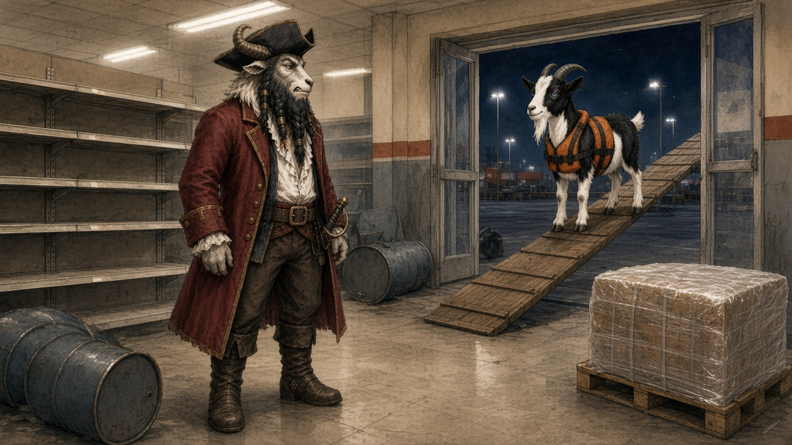
The Crimson Barnacle shuddered as it dropped out of the time-stream and settled into the dim glow of a parking lot somewhere in suburban Earth, March 2020. Captain Pirate Pete had wanted gasoline and diesel. What he found instead was chaos. Two shoppers were fighting over the last shrink-wrapped bale of toilet paper, and a shelf that should have held a hundred packages held exactly none. "Blisterin' barnacles," Pete muttered, "it's the Great Toilet Paper Shortage. We've sailed right into the whirlpool."
Pete planted his boots between the empty shelves and the last bale. "We burned the diesel to get here," he said. "We're buying the paper. Whatever it costs."
Socks called down from the gangplank, hooves ticking on the ramp. "The diesel is burned, Captain. You will not see it again. Spent, and unrecoverable — that is a sunk cost, and it does not get a vote. The next pack is the only decision left. If the price is a panic price, we walk. Coming all this way is not a reason to pay it."
Pete's jaw worked. He did not reach for the bale.
First Mate Orpheus poked his head out from the galley, wiping his hands on his apron. "Captain, I've seen this before. Not the paper — the panic. People will pay anything when they think they can't get a thing. But raise the price of a cup of coffee by a dime and they march off to the competitor down the street. Why does the price of one thing barely move buyers while the price of another sends them stampeding?" Stella Starlight, still half-dreaming of the North Atlantic from which the crew had plucked her, blinked. "You mean some things we just... can't stop buying? That seems terribly unfair."
Socks the GOAT trotted down the gangplank, hooves clicking, navigational instruments slung around his neck. "It isn't fairness, Stella. It's elasticity — the single most useful number in all of economics, and the one the Hypno Hippo most wants you never to learn." At the mention of the villain, a flicker of purple light pulsed from a nearby billboard: a TokPod ad, feeding, always feeding. Petunia Pareto adjusted her spectacles and sighed happily. "Elasticity is just a derivative in disguise. A ratio of percentage changes. Oh, it's beautiful."
Socks fixed the crew with a steady stare. "Today we learn to measure responsiveness. We'll learn why some sellers can double their prices and grow rich, while others try the same and go bankrupt. We'll learn why a tax on cigarettes lands on smokers but a tax on luxury yachts lands on yacht-builders. Pay attention — this is the knowledge that turns a victim of the market into a navigator of it. X marks the spot, but elasticity tells you how hard the current is pulling." And so, in a ransacked big-box store at the dawn of a pandemic, the lecture began.

1. What Elasticity Measures: Responsiveness, Not Slope
Socks the GOAT planted his hooves and began. "The first thing you must unlearn, Stella, is the temptation to say 'how much does quantity change when price changes' in raw units. Units lie. A dollar means one thing for a pack of gum and nothing for a yacht. So economists do not measure responsiveness in units. We measure it in percentages."
1.1 The core definition
The price elasticity of demand answers one question: when the price of a good rises by one percent, by what percentage does the quantity demanded fall? Formally, it is the ratio of the percentage change in quantity demanded to the percentage change in price [3]:
Because the law of demand tells us that price and quantity demanded move in opposite directions, this ratio is almost always negative. By long convention economists drop the minus sign and talk about the absolute value of elasticity, so that a bigger number always means "more responsive." When Socks says demand is "more elastic," he means buyers run away faster when the price climbs.
1.2 Why percentages, not units
Petunia floated over, delighted. "Consider, Stella. Suppose the toilet paper price rises from four dollars to five dollars — that's a twenty-five percent increase. And suppose a yacht's price rises from one million to one million and one dollars. Both went up by roughly the same raw... no wait, they didn't." She caught herself. "The point is that only percentages let us compare a gum market to a yacht market on the same ruler." Because elasticity is a ratio of two percentages, it is a pure number with no units — it is the same whether we price in dollars, doubloons, or the Hippo's dopamine-tokens.
1.3 The three buckets
Socks drew three lines in the dust of the parking lot. Economists sort every good into three buckets based on the absolute value of its elasticity. When \(|E_d| > 1\), demand is elastic: quantity is very responsive, and buyers flee a price hike. When \(|E_d| < 1\), demand is inelastic: quantity barely budges, and buyers grit their teeth and pay. And at the knife's edge, when \(|E_d| = 1\), demand is unit elastic: the percentage change in quantity exactly matches the percentage change in price.
2. The Midpoint Method: Doing the Arithmetic Honestly
"Now," said Socks, "there is a trap in the arithmetic, and the Hypno Hippo loves traps. If you compute percentage change the naive way, you get two different answers depending on whether the price went up or came down. That is nonsense. The responsiveness of a market segment should not depend on which direction you happened to walk along it."
2.1 The problem with ordinary percentage change
Suppose quantity goes from 100 to 150. Using the starting value as the base, that's a 50% increase. But going from 150 back to 100 is only a 33% decrease over the same stretch. Same two points, two different percentages. Petunia frowned. "The derivative doesn't care which direction you approach from. Neither should we." The fix is to divide the change not by the starting value but by the average of the two values — the midpoint.
2.2 The midpoint formula
The midpoint method (also called the arc-elasticity method) computes each percentage change relative to the average of the endpoints:
Because both the numerator and denominator use the midpoint as their base, you get the same elasticity whether you move from point 1 to point 2 or back again. This is the standard the course will use for every calculation.
2.3 A worked calculation
Stella raised her hand. "Could we try a real one? With the toilet paper?" Socks nodded. Imagine that before the panic, a store sold 500 packages a week at $4. During a modest price increase to $5, weekly sales fell to 450. Let's measure.
Midpoint elasticity of toilet paper demand
\(E_d = \frac{(Q_2 - Q_1)/[(Q_2 + Q_1)/2]}{(P_2 - P_1)/[(P_1 + P_2)/2]}\)
| Input | Value | Unit |
|---|---|---|
| Q1 (packages/week) | 500 | pkg |
| Q2 (packages/week) | 450 | pkg |
| P1 (price) | 4 | USD |
| P2 (price) | 5 | USD |
Result: -0.4737 elasticity (unitless)
Walking through it: the quantity change is \(450-500=-50\), and the average quantity is \((450+500)/2=475\), so the percentage change in quantity is \(-50/475 = -0.1053\), or about −10.5%. The price change is \(5-4=1\), and the average price is \((5+4)/2=4.5\), so the percentage change in price is \(1/4.5 = 0.2222\), or about +22.2%. Dividing, \(-0.1053 / 0.2222 = -0.474\). The absolute value, 0.47, is less than one — toilet paper demand in this range is inelastic. "Of course it is," muttered Orpheus. "Nobody shops around for a cheaper substitute when nature calls."
3. Elastic, Inelastic, and Unit Elastic: Three Illustrative Goods
Socks produced a small chalkboard from the Crimson Barnacle's hold. "Let me show you three goods side by side, so you can see responsiveness with your own eyes." These are teaching numbers, chosen to make the three cases crisp.
3.1 Three demand schedules
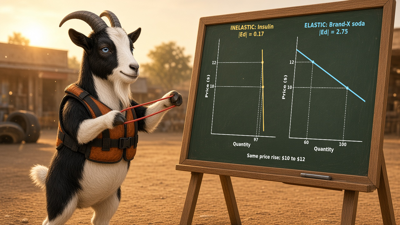
Simplified example: the table below shows three illustrative goods, each facing the same price rise from $10 to $12. Insulin is a near-necessity with no substitute; a mid-range restaurant meal has some substitutes; and a particular brand of soda has many close substitutes. The quantities are pedagogical, not empirical.
| Good | P₁ (USD) | Q₁ (units) | P₂ (USD) | Q₂ (units) | |E_d| (midpoint) | Classification |
|---|---|---|---|---|---|---|
| Insulin (necessity) | 10 | 100 | 12 | 97 | 0.17 | Inelastic |
| Restaurant meal | 10 | 100 | 12 | 82 | 1.00 | Unit elastic |
| Brand-X soda | 10 | 100 | 12 | 60 | 2.75 | Elastic |
For insulin, quantity falls from 100 to 97 — a tiny response to a 20% price hike, giving \(|E_d|\approx 0.17\). For the restaurant meal, quantity falls from 100 to 82, giving an elasticity of almost exactly 1. For Brand-X soda — which buyers will happily abandon for Brand-Y — quantity collapses from 100 to 60, giving \(|E_d|\approx 2.75\).
3.2 Visualizing the three curves
The chart below plots the three demand curves from the table above. Notice that the flatter curve (soda) is the more elastic one over this range, and the steeper curve (insulin) is the more inelastic.
Three Illustrative Demand Curves Over the Same Price Rise
Three downward-sloping demand segments all running from a price of 10 up to a price of 12. The insulin curve barely moves left (quantity 100 to 97), the restaurant meal moves moderately (100 to 82), and the soda curve moves far left (100 to 60), showing that flatter curves over this range are more elastic.
3.3 A caution about slope versus elasticity
4. The Determinants of Elasticity: Why Some Goods Resist Price
Stella was puzzled. "But Socks, how does a buyer decide to be responsive? What makes insulin stubborn and soda flighty?" The goat smiled. "Excellent question. Elasticity is not random. Four forces drive it."
4.1 Substitutes: the master key
The single most important determinant is the availability of close substitutes. If a good has many close substitutes, buyers can switch the moment its price rises, and demand is elastic. If it has none, buyers are trapped and demand is inelastic. This is why a particular brand of soda is far more elastic than soda in general, which is in turn more elastic than all beverages. The narrower you draw the category, the more substitutes exist outside it, and the more elastic demand becomes.
4.2 Necessities versus luxuries
Goods that feel like necessities — insulin, basic food, home heating — tend to be inelastic, because buyers cut other spending before they cut these. Luxuries — exotic vacations, designer handbags, a second yacht — tend to be elastic, because they are the first things abandoned when the price climbs. "The Hypno Hippo," Socks added darkly, "works very hard to make his TokPods feel like necessities. An addiction is just a demand curve he has bent to vertical."
4.3 Share of the budget
A good that eats a large share of your budget is one you watch closely; a price rise there forces you to respond. A trivial purchase — a pack of salt, a box of toothpicks — can double in price without most buyers noticing, so demand is inelastic. The larger the budget share, the more elastic the demand tends to be.
4.4 Time horizon
The longer the time horizon, the more ways buyers find to substitute away, and the more elastic demand becomes. A short-run elasticity and a long-run elasticity for the very same good can differ by a factor of three or more.
5. Elasticity Along a Straight-Line Demand Curve
"Now I will show you the thing that trips up half of all students," said Socks, "and I will show it with a picture." Petunia was already vibrating with excitement at the prospect of a changing derivative.
5.1 The paradox of the straight line
A straight-line (linear) demand curve has a constant slope. One might therefore assume it has a constant elasticity. It does not. Elasticity depends not only on the slope \(\Delta P / \Delta Q\) but on the ratio of price to quantity at the point you're measuring. The relationship between the slope and elasticity runs through the demand slope:
At the top of the demand curve, price is high and quantity is low, so the price-to-quantity ratio is enormous and elasticity is large (elastic). At the bottom, price is low and quantity is high, so the ratio is tiny and elasticity is small (inelastic). Somewhere in the middle, elasticity passes through exactly 1 — unit elastic.
5.2 A worked midpoint at two ends
Consider a simple linear demand curve. Simplified example: let the demand be \(Q = 100 - 10P\). Up near the top, move price from $8 to $9 (quantity from 20 to 10). Down near the bottom, move price from $2 to $3 (quantity from 80 to 70).
Elasticity near the top of a linear demand curve
\(E_d = \frac{(Q_2 - Q_1)/[(Q_2 + Q_1)/2]}{(P_2 - P_1)/[(P_1 + P_2)/2]}\)
| Input | Value | Unit |
|---|---|---|
| Q1 at P=8 | 20 | units |
| Q2 at P=9 | 10 | units |
| P1 | 8 | USD |
| P2 | 9 | USD |
Result: -5.67 elasticity (unitless)
Near the top: \(\%\Delta Q = -10/15 = -0.667\); \(\%\Delta P = 1/8.5 = 0.1176\); ratio \(= -5.67\). Strongly elastic. Now the bottom:
Elasticity near the bottom of a linear demand curve
\(E_d = \frac{(Q_2 - Q_1)/[(Q_2 + Q_1)/2]}{(P_2 - P_1)/[(P_1 + P_2)/2]}\)
| Input | Value | Unit |
|---|---|---|
| Q1 at P=2 | 80 | units |
| Q2 at P=3 | 70 | units |
| P1 | 2 | USD |
| P2 | 3 | USD |
Result: -0.33 elasticity (unitless)
Near the bottom: \(\%\Delta Q = -10/75 = -0.1333\); \(\%\Delta P = 1/2.5 = 0.40\); ratio \(= -0.33\). Strongly inelastic. Same curve, same slope, utterly different elasticity.
5.3 The linear demand and supply set
To anchor this, here is a simple linear demand-and-supply pair we'll reuse. Simplified example: demand \(Q_d = 100 - 10P\) and supply \(Q_s = -20 + 20P\). Setting them equal gives equilibrium at \(P=4\), \(Q=60\). The table below traces the demand curve and marks where elasticity transitions.
| Price (USD) | Qd = 100 − 10P (units) | Qs = −20 + 20P (units) | Demand region |
|---|---|---|---|
| 9 | 10 | 160 | Elastic |
| 7 | 30 | 120 | Elastic |
| 5 | 50 | 80 | ~Unit elastic region |
| 4 | 60 | 60 | Equilibrium |
| 3 | 70 | 40 | Inelastic |
| 1 | 90 | 0 | Inelastic |
Linear Demand and Supply with Equilibrium at P=4, Q=60
A downward-sloping linear demand line and an upward-sloping linear supply line crossing at a price of 4 and quantity of 60. The demand line is elastic at high prices (upper left) and inelastic at low prices (lower right).
6. Elasticity and Total Revenue: The Seller's Compass
Orpheus leaned in. "This is the part that matters for a working sailor. If I'm selling fish on the dock, should I raise my price or lower it to make more coin?" Socks grinned. "Elasticity answers exactly that. It is a seller's compass."
6.1 Total revenue defined
Total revenue is simply price times quantity sold: \(TR = P \times Q\). When a seller raises the price, two forces fight. The price effect pushes revenue up (each unit sells for more). The quantity effect pushes revenue down (fewer units sell). Which wins depends entirely on elasticity.
6.2 The total revenue rule
When demand is inelastic (\(|E_d|<1\)), quantity barely falls when price rises, so the price effect dominates: raising price raises total revenue. When demand is elastic (\(|E_d|>1\)), quantity falls sharply, so the quantity effect dominates: raising price lowers total revenue. And at unit elasticity, the two effects exactly cancel and total revenue is at its maximum.

6.3 A worked revenue table
Using our demand curve \(Q = 100 - 10P\), let's compute total revenue at each price and watch it rise, peak, then fall.
| Price (USD) | Quantity (units) | Total Revenue = P×Q (USD) | Demand over this range |
|---|---|---|---|
| 9 | 10 | 90 | Elastic |
| 8 | 20 | 160 | Elastic |
| 7 | 30 | 210 | Elastic |
| 6 | 40 | 240 | Elastic |
| 5 | 50 | 250 | Unit elastic (peak) |
| 4 | 60 | 240 | Inelastic |
| 3 | 70 | 210 | Inelastic |
| 2 | 80 | 160 | Inelastic |
| 1 | 90 | 90 | Inelastic |
Total revenue at the unit-elastic peak
\(TR = P \times Q\)
| Input | Value | Unit |
|---|---|---|
| Price | 5 | USD |
| Quantity | 50 | units |
Result: 250 USD
Total Revenue Peaks at the Unit-Elastic Price
A hump-shaped total revenue curve rising from 90 at a price of 9 up to a peak of 250 at a price of 5, then falling back to 90 at a price of 1. The peak coincides with unit-elastic demand.
6.4 The fish connection
Petunia clapped. "It's the fish again! Revenue humped like a well-fed fish, fattest in the middle where elasticity equals one." Socks nodded — the crew had seen this shape before, hunting the elusive maximum where marginal revenue meets marginal cost. "At the top of this revenue hump, raising the price one more cent costs you exactly as much in lost quantity as it gains you in margin. That is unit elasticity, and it is where a revenue-maximizing seller plants her flag."
Socks glanced at Stella. "That next cent is the margin: judge the unit still in front of you, and keep a substitute in mind so you can still refuse it."
7. Cross-Price and Income Elasticity: Mapping the Web of Goods
"Price elasticity is only the first of a family," said Socks. "Two cousins tell you how a good relates to other goods and to income."
7.1 Cross-price elasticity
The cross-price elasticity of demand measures how the quantity demanded of one good responds to a price change in another good:
The sign tells you the relationship. If \(E_{XY}>0\), the goods are substitutes: when coffee's price rises, people buy more tea (tea quantity up, coffee price up — same direction, positive). If \(E_{XY}<0\), the goods are complements: when printers get more expensive, people buy fewer ink cartridges (cartridge quantity down, printer price up — opposite direction, negative). If near zero, the goods are unrelated.
Cross-price elasticity of tea with respect to coffee
\(E_{XY} = \frac{\%\Delta Q_X}{\%\Delta P_Y}\)
| Input | Value | Unit |
|---|---|---|
| % change in quantity of tea | 15 | % |
| % change in price of coffee | 30 | % |
Result: 0.5 elasticity (unitless)
A cross-price elasticity of +0.5 means tea and coffee are substitutes, but mild ones — a 30% jump in coffee's price only nudges tea purchases up 15%.
7.2 Income elasticity
The income elasticity of demand measures how quantity demanded responds to a change in income. If positive, the good is normal (you buy more as you get richer). If large and positive (greater than 1), it's a luxury. If negative, it's an inferior good (you buy less as you get richer — think instant ramen replaced by restaurant meals).
Income elasticity of restaurant meals
\(E_I = \frac{\%\Delta Q}{\%\Delta M}\)
| Input | Value | Unit |
|---|---|---|
| % change in quantity demanded | 24 | % |
| % change in income | 12 | % |
Result: 2 elasticity (unitless)
An income elasticity of 2.0 means restaurant meals are a luxury: a 12% rise in income produces a 24% rise in restaurant dining. Note we reuse the same ratio-of-percentages machinery as Eq. 1 — only the denominator changes from price to income.
8. Tax Incidence: Who Really Pays Depends on Elasticity
Vilfredo Vitriol, lurking at the edge of the parking lot, sneered at the mention of taxes — he had made fortunes by knowing who would truly bear them. "You children," he drawled, "think a tax falls on whoever the law names. How quaint." Socks did not take the bait; he simply taught.
8.1 Statutory versus economic incidence
Tax incidence is the study of who actually bears the burden of a tax, which is often very different from who legally writes the check. The law can require sellers to remit a tax, but sellers raise their prices to pass part of it to buyers. The economic incidence — the real burden — is decided not by the legislature but by relative elasticity.
8.2 The incidence rule
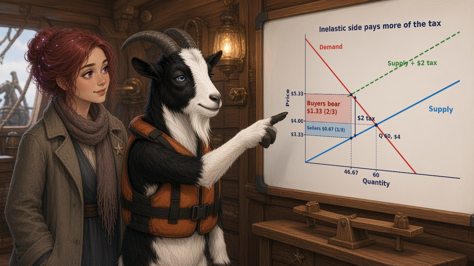
The core result: the more inelastic side of the market bears more of the tax. If buyers can't easily leave (inelastic demand), they get stuck with most of the burden. If sellers can't easily exit (inelastic supply), they eat most of it. Intuitively, whoever can most easily walk away from the transaction escapes the tax; whoever is trapped pays.
8.3 Why cigarette and yacht taxes land so differently
8.4 A worked incidence split
Simplified example: suppose a $2 per-unit tax is imposed in the §5.3 market, where demand is \(Q_d = 100 - 10P\) and supply is \(Q_s = -20 + 20P\), so the pre-tax equilibrium is \(P = 4\), \(Q = 60\). After the tax, the price buyers pay rises from $4.00 to $5.33, while the price sellers keep falls from $4.00 to $3.33, and quantity falls from 60 to about 46.67.
Buyer's share of a per-unit tax
\(\frac{\text{rise in the buyer price}}{\text{tax}}\)
| Input | Value | Unit |
|---|---|---|
| Rise in buyer price | 1.33 | USD |
| Total tax per unit | 2 | USD |
Result: 0.67 share (unitless)
The buyer price rose by $1.33 of the $2.00 tax, so buyers bear two-thirds of the burden and sellers bear the remaining one-third (the $0.67 drop in what they keep). This split tells us demand here is more inelastic than supply — buyers were the more trapped side. It matches the incidence rule: at \(P = 4\), \(Q = 60\), \(|E_d| = 10 \times 4/60 \approx 0.67\) and \(E_s = 20 \times 4/60 \approx 1.33\), so the buyers' share is \(E_s/(E_s + |E_d|) = 1.33/2 = 2/3\).
9. Real Inflation Data: Reading the CPI Through an Elasticity Lens
Socks pulled a dusty ledger from the Barnacle. "Before we leave 2020, let me connect elasticity to a number you'll hear every month: the price level itself. The Bureau of Labor Statistics [5] tracks the Consumer Price Index — the average price of a basket of goods. Watching it rise tells us how much the cost of living climbs; watching how buyers respond is where elasticity lives."
9.1 The CPI series
The table below shows the U.S. Consumer Price Index for All Urban Consumers (series CUUR0000SA0), December values, drawn from the Bureau of Labor Statistics [5]. These are index numbers, not dollars; they measure the price level relative to the 1982–84 base of 100.
| Year (December) | CPI-U (CUUR0000SA0), index 1982–84=100 |
|---|---|
| 2015 | 236.525 |
| 2016 | 241.432 |
| 2017 | 246.524 |
| 2018 | 251.233 |
| 2019 | 256.974 |
| 2020 | 260.474 |
| 2021 | 278.802 |
| 2022 | 296.797 |
| 2023 | 306.746 |
| 2024 | 315.605 |
U.S. CPI-U, December Values 2015–2024 (BLS CUUR0000SA0)
A line chart of the Consumer Price Index for All Urban Consumers, December values, rising steadily from 236.525 in 2015 to 260.474 in 2020, then climbing more steeply to 315.605 by 2024.
9.2 The inflation connection
The year-over-year change in this index is the inflation rate, computed as the percentage change from one December to the next:
December-to-December CPI inflation, 2021 over 2020
\(\frac{P_t - P_{t-1}}{P_{t-1}} \times 100\)
| Input | Value | Unit |
|---|---|---|
| CPI Dec 2021 | 278.802 | index |
| CPI Dec 2020 | 260.474 | index |
Result: 7.04 %
From December 2020 to December 2021 the index rose from 260.474 to 278.802, an increase of about 7.0%. "Here is the elasticity lesson," said Socks. "When the price level jumps like this, households respond differently for different goods. For inelastic necessities — food staples, rent, medicine — they keep buying and simply feel poorer. For elastic goods, they substitute or cut back. The pain of inflation is distributed exactly according to elasticity. The Hypno Hippo prospers in such confusion, because a population that can't read the CPI can't tell real pain from engineered panic."
10. Elasticity Across the Centuries: From 1625 to 2425
As the lesson wound down, the Crimson Barnacle's time-engine thrummed, and the crew glimpsed how elasticity echoes across the ages. "This is why we sail through time," Pete said. "The principle is eternal; only the goods change."
10.1 1625: the mercantilist salt trade
In 1625, salt was the great inelastic good — the only way to preserve food through winter, with no substitute. Rulers taxed it mercilessly (the infamous salt taxes of the era) precisely because its inelastic demand made the revenue reliable and the burden fell squarely on the common buyer. A monopolist or a monarch who understands inelasticity can extract enormous rents; a population that doesn't understand it simply pays.

10.2 2025: digital goods and the Hippo's engineered inelasticity
In the present, the most valuable business skill is manufacturing inelasticity. Lock-in, network effects, and addiction all do the same thing: they strip away substitutes and bend the demand curve toward vertical. The Hypno Hippo's TokPods are the purest case — a good engineered so that users cannot walk away, which lets him raise the "price" (in time and attention) without losing the audience.
10.3 2425: the only defense
Stella Starlight looked up at the purple TokPod billboard, then back at Socks, and for the first time she did not feel dreamy or clueless. She felt responsive. "So if I always keep a substitute in mind," she said slowly, "no one can ever trap me." Socks nodded. "Now you're navigating, lass. Now you read the scoreboard." And the Crimson Barnacle lifted off, bound for the next century, its goat-skull sail catching the light.
Key Takeaways
- Price elasticity of demand measures responsiveness as a ratio of percentage changes (%ΔQ over %ΔP), making it a unitless number that compares any two markets on the same ruler.
- Demand is elastic when |E_d| > 1 (buyers flee price hikes), inelastic when |E_d| < 1 (buyers stay), and unit elastic when |E_d| = 1 (the two percentage changes match).
- Always use the midpoint method so the elasticity is the same whether price rises or falls; it divides each change by the average of the endpoints.
- Four determinants drive elasticity: availability of close substitutes (the master key), necessity versus luxury, share of the budget, and the time horizon.
- The total revenue rule: raise price when demand is inelastic, cut price when demand is elastic, and revenue is maximized at unit elasticity.
- Cross-price elasticity reveals substitutes (positive) and complements (negative); income elasticity reveals normal, luxury, and inferior goods.
- Tax incidence falls on the more inelastic side of the market — whoever can least easily walk away bears the heaviest burden, regardless of who the law names.
Check Yourself
Check Yourself 1: Classify from a midpoint calculation
Scenario: A coffee cart sells 200 cups a day at $3. When it raises the price to $4, sales fall to 120 cups.
Question: Compute the midpoint elasticity and classify this demand as elastic, inelastic, or unit elastic.
Reveal worked answer
Answer: The quantity change is \(120-200=-80\) with average \((120+200)/2=160\), so \(\%\Delta Q = -80/160 = -0.50\). The price change is \(4-3=1\) with average \(3.5\), so \(\%\Delta P = 1/3.5 = 0.286\). Dividing, \(E_d = -0.50/0.286 = -1.75\). The absolute value, 1.75, exceeds 1, so demand is elastic — customers have nearby substitutes (another cart, tea, no coffee at all) and flee the price hike.
Check Yourself 2: Predict the revenue move
Scenario: A subway system finds that ridership barely changes when fares rise — its elasticity is about 0.3.
Question: If the city wants more fare revenue, should it raise or lower fares? Explain using the total revenue rule.
Reveal worked answer
Answer: With |E_d| = 0.3 < 1, demand is inelastic, so the price effect dominates the quantity effect. Raising fares will raise total revenue because the small drop in ridership is more than offset by the higher fare on each remaining rider. The city should raise fares to increase revenue (though equity and congestion goals may argue otherwise — revenue is not the only objective).
Check Yourself 3: Read a cross-price sign
Question: The price of e-readers falls 20% and the quantity of printed books demanded falls 8%. Compute the cross-price elasticity and state whether the goods are substitutes or complements.
Reveal worked answer
Answer: \(E_{XY} = \%\Delta Q_{books} / \%\Delta P_{ereaders} = (-8\%)/(-20\%) = +0.4\). The sign is positive, so printed books and e-readers are substitutes: cheaper e-readers lure buyers away from printed books. The magnitude of 0.4 says the substitution is real but moderate.
Check Yourself 4: Who bears the tax?
Scenario: Insulin has very inelastic demand; the supply of insulin is relatively elastic. A government places a per-unit tax on insulin.
Question: Who bears most of the tax burden, and why?
Reveal worked answer
Answer: Buyers bear most of the burden. The incidence rule says the more inelastic side pays more, because it is the side least able to walk away. Insulin buyers cannot substitute away or quit, so sellers pass most of the tax forward into the price patients pay. The elastic supply side can more easily reduce quantity, escaping much of the tax. This is exactly why taxes on inelastic necessities raise reliable revenue but can fall hardest on the vulnerable.
Check Yourself 5: Why does elasticity change along a straight line?
Question: A classmate insists that because a linear demand curve has constant slope, it must have constant elasticity. Correct the misconception.
Reveal worked answer
Answer: Slope uses raw units (ΔP/ΔQ) and is indeed constant on a straight line, but elasticity uses percentages and depends on the price-to-quantity ratio at the measuring point. Near the top, price is high and quantity low, so a 1-unit price change is a small percentage while a 1-unit quantity change is a large percentage — demand is elastic. Near the bottom, the reverse holds and demand is inelastic. The same curve runs from elastic at the top through unit-elastic in the middle to inelastic at the bottom.
Discussion Questions
- The Hypno Hippo's TokPods are described as "engineered inelasticity." Using the four determinants of elasticity, explain precisely which levers a company pulls to make its product's demand more inelastic — and what a critical-thinking defense against each lever would look like.
- In 1625 rulers taxed salt heavily because its demand was inelastic. Compare the salt tax to the modern cigarette tax and the failed luxury yacht tax from the lecture. Why did two of these raise reliable revenue while the third collapsed its own tax base? What does this teach about choosing what to tax?
- Socks tells Stella that keeping a substitute in mind means "no one can ever trap you." Translate this piece of pirate wisdom into the formal language of elasticity and tax incidence. In what sense is an economically literate consumer always on the "elastic" side of every market, and why does that protect them?
Glossary
- price elasticity of demand
- A measure of how responsive the quantity demanded of a good is to a change in its price, expressed as the ratio of the percentage change in quantity to the percentage change in price.
- law of demand
- The principle that, all else equal, the quantity demanded of a good falls as its price rises.
- absolute value
- A number's magnitude without regard to sign; used so that larger elasticity values always indicate greater responsiveness.
- elastic
- Demand for which the absolute value of elasticity exceeds one, meaning quantity responds more than proportionally to a price change.
- inelastic
- Demand for which the absolute value of elasticity is less than one, meaning quantity responds less than proportionally to a price change.
- unit elastic
- Demand for which the absolute value of elasticity equals one, so the percentage change in quantity exactly matches the percentage change in price.
- percentages
- Relative changes expressed per hundred, used in elasticity so that goods measured in different units can be compared on a common scale.
- midpoint method
- A technique for computing elasticity that divides each change by the average of the two endpoint values, so the result is the same in either direction.
- availability of close substitutes
- The degree to which other goods can replace a given good; the primary determinant of how elastic its demand is.
- time horizon
- The length of time buyers have to adjust to a price change; longer horizons generally make demand more elastic.
- demand slope
- The change in price divided by the change in quantity along a demand curve, measured in raw units rather than percentages.
- total revenue
- The total receipts of a seller, equal to price multiplied by quantity sold.
- total revenue rule
- The principle that raising price increases total revenue when demand is inelastic and decreases it when demand is elastic, with revenue maximized at unit elasticity.
- cross-price elasticity of demand
- A measure of how the quantity demanded of one good responds to a change in the price of another good; its sign indicates whether the goods are substitutes or complements.
- substitutes
- Goods that can replace one another, so that a rise in the price of one increases demand for the other, giving a positive cross-price elasticity.
- complements
- Goods consumed together, so that a rise in the price of one decreases demand for the other, giving a negative cross-price elasticity.
- income elasticity of demand
- A measure of how quantity demanded responds to a change in consumer income, used to classify goods as normal, luxury, or inferior.
- normal
- A good whose quantity demanded rises as consumer income rises, giving a positive income elasticity.
- luxury
- A normal good with income elasticity greater than one, so demand rises more than proportionally with income.
- inferior good
- A good whose quantity demanded falls as consumer income rises, giving a negative income elasticity.
- tax incidence
- The analysis of who actually bears the economic burden of a tax, which depends on relative elasticities rather than on who legally pays.
- inflation rate
- The percentage change in the general price level from one period to the next.
References
- (2015). Elasticity of Demand. https://learn.mru.org/courses/principles-of-microeconomics/units/elasticity-and-its-applications/lessons/elasticity-demand-definition
- (2015). Calculating the Elasticity of Demand. https://learn.mru.org/courses/principles-of-microeconomics/units/elasticity-and-its-applications/lessons/calculate-elasticity-demand-formula
- (2021). Modern Principles: Microeconomics. Worth Publishers
- (2012). Demand for gasoline is more price-inelastic than commonly thought. Elsevier BV. https://doi.org/10.1016/j.eneco.2011.09.003
- (2026). Consumer Price Index for All Urban Consumers (CPI-U): All Items in U.S. City Average, Not Seasonally Adjusted (CUUR0000SA0). U.S. Bureau of Labor Statistics. https://data.bls.gov/timeseries/CUUR0000SA0