Lecture

The Law of Demand

Why Are You So Demanding?

Watch first: Jacob Clifford's walk-through of the law of demand and shifts versus movements ^[1], and Crash Course Economics #4 on supply and demand ^[2].

The Crimson Barnacle, a wooden space-time pirate galleon with limp crimson sails and one goat-skull sail, sits motionless in a glowing teal-and-amber cosmic calm with a faint distant time-tunnel on the horizon. — Becalmed in the glowing doldrums: the Crimson Barnacle sits dead-still, waiting — the perfect moment to ask what people are willing to pay.

Three weeks becalmed in the glowing doldrums of Omni Cron 72 will test any crew. The Crimson Barnacle sat dead in the cosmic water, her time-sails limp, her engines waiting for the sun to drift past the mouth of the tunnel. Petunia Pareto clip-clopped across the deck in a fury, round spectacles fogging, because Stella Starlight—the dreamy auburn-haired girl they had fished out of the freezing Atlantic in 1912—had once again spent the entire morning thumb-scrolling a Hypno Hippo TokPod instead of studying.

"Why," Stella groaned, flopping dramatically over a coil of rope, "does an orphan from Ireland need to learn economics? I almost froze to death in the North Atlantic. I think I've earned a nap."

Petunia's eyes flashed. "We are a pirate ship with a G.O.A.T. crew. Economics is what we DO. Every supply run, every treasure, every jump through time—it all comes down to one question: what are people willing to pay, and what does it cost us to provide it? Get that wrong and we end up stranded in the wrong century with an empty hold. You remember what happened to the people who misjudged the North Atlantic."

Stella went quiet. Petunia softened—she knew a working-class kid from 1912 Ireland had barely seen a schoolroom. So she pushed her spectacles up her nose and dragged a parchment easel across the deck. "Our next stop is Earth 2020, right?" she called to Socks the GOAT, the ship's navigator. Socks nodded: "Costco run. Toilet paper, diesel, oats, rum, coffee, insulin—pirate essentials." Petunia smiled. If she could teach Stella to read a demand curve before they hit the aisles of the Great Toilet Paper Shortage, the girl would never go hungry in the wrong century again. She picked up a stick of chalk. "All right, Stella," she said. "Let me show you how price and quantity dance."

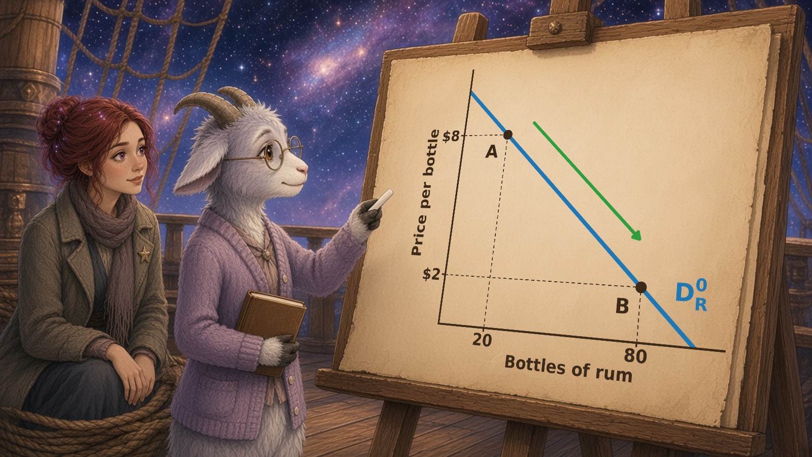
Petunia Pareto, a lilac-grey goat in round spectacles and a lilac cardigan, holds up chalk beside a large parchment easel on the ship's deck at night while Stella Starlight watches from a coil of rope. The parchment shows the original rum demand curve, D-zero-R, as a blue line sloping down. Point A is at $8 and 20 bottles and point B is at $2 and 80 bottles, with thin dashed drop lines to both axes and a green arrow from A to B for the price fall. — Petunia's law of demand: when the price of rum falls from $8 to $2 (A to B along $D^{0}_{R}$), the quantity demanded rises from 20 to 80 bottles.

1. The Law of Demand: Why Price and Quantity Pull Against Each Other

Petunia tapped the chart with her hoof. "Here's the first and oldest law of the market, Stella. Hold everything else fixed—your income, your tastes, the prices of everything else—and ask only this: when the price of a thing goes up, what happens to the quantity people want to buy?" Stella thought about the TokPod store, where a "premium emoji pack" had just doubled in price. "I'd buy less of it," she admitted. "Exactly," said Petunia. "That is the law of demand: as price rises, the quantity demanded falls, and as price falls, quantity demanded rises. Price and quantity move in opposite directions."

1.1 Why the law holds — two forces under the hood

The law of demand is not a mysterious decree; it falls out of how real people make choices. There are two reasons buyers retreat when prices climb. The first is the substitution effect: when coffee gets expensive, tea and energy drinks suddenly look like better deals, and some coffee drinkers switch. The second is the income effect: when a price rises, each dollar in your pocket stretches over fewer goods, so your real purchasing power shrinks and you simply buy less of almost everything. Cowen and Tabarrok build the entire demand curve from these micro-foundations—ultimately from marginal utility and the budget a consumer faces ^[3].

Petunia, who sees the world in derivatives, went one layer deeper. "The deepest root is diminishing marginal utility. The first cup of rum on a cold voyage is glorious. The fourth is... less so. Because each additional unit gives you less extra satisfaction, you are only willing to pay a lower price for additional units. That is why the willingness-to-pay schedule slides downward as quantity rises." The extra satisfaction from one more unit is captured by marginal utility,

\[MU_X = \frac{\Delta TU}{\Delta X}\]

(1)

and because that number shrinks as you consume more, your willingness to pay shrinks with it. ^[3]

Socks the goat in his orange life vest sits at a galley counter with four tankards in a row, from drained to untouched, nudging the fourth one away. — The first mug is worth a lot; the fourth is worth almost nothing. Each extra unit adds less: diminishing marginal utility.

1.2 Willingness-to-pay: reading the curve the other way

Here is the move that unlocks everything for a pirate crew. A demand curve can be read in two directions. Read horizontally—pick a price, read off the quantity—it tells you how much people will buy at a given price. Read vertically—pick a quantity, read off the price—it tells you the maximum price someone is willing to pay for that particular unit. For the Crimson Barnacle, which survives by buying low in one century and selling high in another, the vertical reading is the whole game. If Socks can read off what a 2020 shopper will pay for the tenth roll of toilet paper, he knows exactly where to set the price. Every price is really a trade-off: with one coin, Pete's rum costs him the cutlasses he can't also buy.

On a sunny harbor dock, Captain Pirate Pete, a goat in a crimson coat and tricorn with a long braided black beard, holds up a single gold coin and reaches longingly for rum bottles, while Socks the goat in his orange life vest sternly points at a rack of cutlasses and a brass cannon, and a cheerful merchant behind the stall waits to be paid. — One coin: rum or cutlasses? Whatever Pete buys, the other is the opportunity cost, and that trade-off is what his willingness to pay measures.

1.3 Quantity demanded is a schedule, not a number

A crucial habit: "demand" is not a single number, it is an entire schedule—a list of price–quantity pairs. When Stella says "the demand for rum," she means the whole relationship across every possible price, not one quantity. The specific amount bought at one specific price has its own name: quantity demanded. Confusing the two is the single most common error in this course, and it is the source of the shift-versus-movement trap we meet in Section 3.

2. Building a Demand Curve: Schedule, Equation, and Graph

Petunia refused to let Stella memorize anything she could not build. "A demand curve," she said, "lives in three bodies: a table, an equation, and a graph. They are the same creature wearing three coats. Learn to translate between them and you will never be fooled."

2.1 From a demand schedule to a graph

Suppose the crew is pricing bottles of rum to trade on a backwater moon. Petunia surveys the locals and writes down how many bottles they would buy at each price.

Simplified example: rum demand schedule (classroom data, not real)

Price (space-credits per bottle)	Quantity demanded (bottles)
10	0
8	20
6	40
4	60
2	80
0	100

Plot these points with price on the vertical axis and quantity on the horizontal axis—the convention economists have used since Alfred Marshall ^[4]—and you get a straight downward-sloping line.

Rum demand as a line

The rum demand schedule plotted as a straight blue line D0 from price 10 at 0 bottles to price 0 at 100 bottles, with dots at (20, 8), (40, 6), (60, 4) and (80, 2).

The rum schedule as a line: every dot is one row of the table.

2.2 From the graph to an equation

Every straight line can be written $P = a - bQ$, where $a$ is the vertical intercept (the choke price, the price so high that quantity demanded falls to zero) and $b$ is the magnitude of the slope. From the table, when $Q = 0$, $P = 10$, so $a = 10$. To get $b$, use the slope of a line, the ratio of rise to run between any two points.

\[\text{slope} = \frac{\Delta P}{\Delta Q} = \frac{P_2 - P_1}{Q_2 - Q_1}\]

(2)

^[3]

Slope of the rum demand line

$\frac{P_2 - P_1}{Q_2 - Q_1}$

Inputs
Input	Value	Unit
P_2	2	credits
P_1	8	credits
Q_2	80	bottles
Q_1	20	bottles

Result: -0.1 credits per bottle

The slope is $-0.1$: every extra bottle the crew tries to sell requires the price to fall by one-tenth of a credit. So the inverse demand equation is $P = 10 - 0.1Q$. Rearranged to put quantity on the left—the "quantity demanded as a function of stuff" form that matches how Petunia actually plans a run—it becomes $Q = 100 - 10P$.

2.3 Demand as a function of everything that matters

Petunia loves to write demand in its fullest form, because it reminds you of everything we are holding fixed when we draw a single curve. Quantity demanded of good X depends not only on its own price but on income, tastes, and the prices of other goods:

\[Q_X = f(P_X,\; M,\; T,\; P_{\text{related}})\]

(3)

In this general demand function, $P_X$ is the good's own price (the endogenous variable we vary along a single curve), while income $M$, tastes $T$, and related-good prices $P_{\text{related}}$ are the exogenous shifters we hold still. The moment any of those shifters moves, we do not slide along the curve—we draw a new curve. That is the heart of Section 3.

3. The Great Trap: Shift of the Curve vs. Movement Along It

Stella looked at the two forms of the rum equation and asked the question that every student eventually asks: "If the price going down makes people buy more... isn't that the demand going up?" Petunia set down her chalk. "This," she said gravely, "is the reef that wrecks more students than any shoal in the galaxy. Let us navigate it carefully."

3.1 Movement ALONG the curve — a change in the good's own price

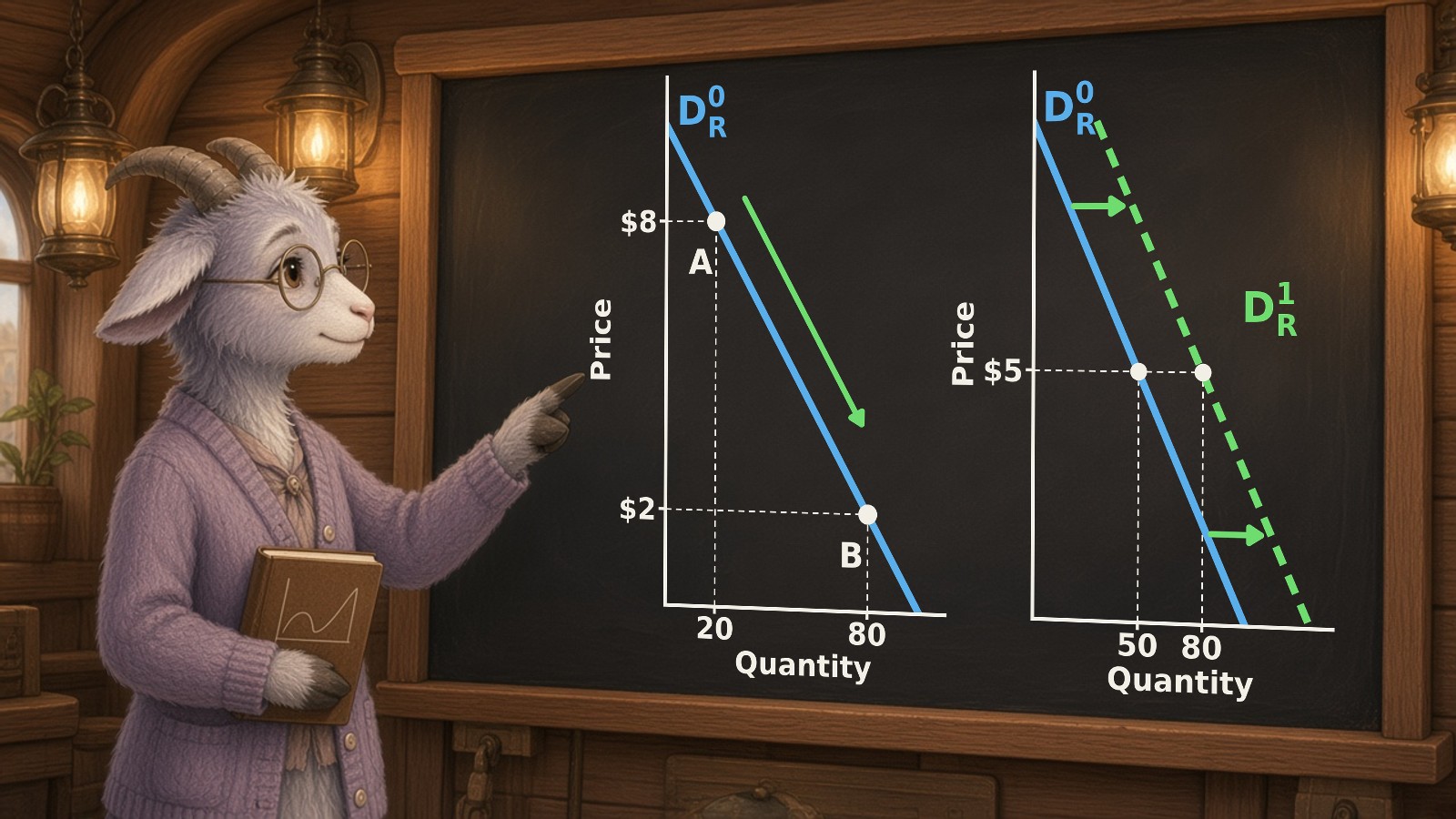
When only the good's own price changes, you do not get a new curve. You slide from one point on the existing curve to another point on the same curve. We call this a change in quantity demanded (notice: quantity demanded, not demand). The rum became cheaper, so buyers slid down to a larger quantity. The line itself never moved. It is a movement along the demand curve.

Movement ALONG the demand curve

One blue rum demand line D0. Point A (P = 8, Q = 20) in blue and point B (P = 2, Q = 80) in green, with a green arrow sliding down the same line; dotted drop lines mark 8, 2, 20 and 80 on the axes.

Only rum's own price fell (green: good for buyers), so buyers slide from A to B on the SAME line: a change in quantity demanded.

The two highlighted points both come from the rum schedule table in Section 2.1.

3.2 Shift OF the curve — a change in an exogenous determinant

Now suppose something other than the rum price changes—say the moon's population doubles, or a new fad makes rum fashionable. At every price, people now want more. The whole schedule moves rightward. This is a change in demand itself: a demand shift. A rightward shift is an increase in demand; a leftward shift is a decrease in demand.

Simplified example: rum demand before and after a rightward shift

Price (credits)	Original quantity (bottles)	After rightward shift (bottles)
10	0	30
8	20	50
6	40	70
4	60	90
2	80	110
0	100	130

Shift OF the demand curve

Two parallel rum demand lines: D0 (blue, Q = 100 − 10P) and D1 (red, dashed, Q = 130 − 10P), 30 bottles to the right at every price. At a price of 6, quantity demanded rises from 40 to 70.

More buyers or a fad (red: rum gets pricier for each buyer) moves the WHOLE line 30 bottles right: an increase in demand.

Notice the new equation. The original was $Q = 100 - 10P$. Adding 30 bottles at every price gives $Q = 130 - 10P$: the slope term $-10$ is unchanged (the curve's steepness is the same), but the intercept grew. That is the algebraic fingerprint of a parallel shift—the constant changes, the slope does not.

Petunia Pareto, a lilac-grey goat in round spectacles and a lilac cardigan, points at a large chalkboard with two panels. Left: a movement along the blue rum demand curve D-zero-R, where a green arrow takes the dot from A ($8, 20 bottles) to B ($2, 80 bottles). Right: a shift of demand, where higher income moves the whole curve right from D-zero-R (solid blue) to D-one-R (dashed green); at $5, quantity demanded rises from 50 to 80 bottles. — Did the dot move, or the line? Left: rum's own price falls, so we slide along $D^{0}_{R}$ from A to B. Right: incomes rise, so at every price buyers want more rum and demand shifts right from $D^{0}_{R}$ to $D^{1}_{R}$ (at $5, from 50 to 80 bottles).

3.3 Why the distinction is life-or-death for pirates

"Here is why I care," said Petunia. "If the price of diesel at Costco falls and we buy more, nothing has changed about the world's appetite for diesel—we just slid down a curve. Now suppose a war breaks out. Most people assume a war makes the world want more diesel. It doesn't. Truckers, farmers, and freighter captains need about as much diesel the day after the shooting starts as the day before. What a war wrecks is supply: oil fields and refineries get hit, and tankers will not sail through a war zone. Fewer barrels reach the market at every price, so the supply curve—the sellers' side of the market, which we will build properly next time—shifts left."

"At the old price there is suddenly a shortage," she went on. "Buyers still want the same amount, but there is less to sell. So the price climbs, and as it climbs we slide up a demand curve that never moved, until the buyers who can do without diesel drop out. And in the short run, diesel demand is steep. You cannot convert a truck or a tractor to run on rum overnight, so demand is inelastic, and a modest loss of barrels sends the price soaring."

War cuts diesel supply

Steep short-run diesel demand D0 (blue, Q = 60 − 2P) does not move. Supply S0 (blue, Q = 10P) shifts left to S1 (red, dashed, Q = 10P − 30) because war hits oil fields, refineries and shipping. Equilibrium slides along the unchanged demand curve from E0 (P = 5, Q = 50) to E1 (P = 7.5, Q = 45).

War cuts supply (red: bad for buyers): S shifts left from S⁰ to S¹, and the price climbs from P⁰ to P¹ along the SAME steep demand curve.

Stella frowned. "So the price went up, but demand didn't?"

"Not one bit," said Petunia. "Quantity demanded fell, because the price rose. Demand stayed exactly where it was. It works in reverse, too: when the shipping lanes reopen, supply shifts back to the right and the price falls along the same demand curve."

Shipping lanes reopen

Steep short-run diesel demand D0 (blue, Q = 60 − 2P) does not move. Supply S0 (blue, Q = 10P) shifts right to S1 (green, dashed, Q = 30 + 10P) because tankers sail again. Equilibrium slides along the unchanged demand curve from E0 (P = 5, Q = 50) to E1 (P = 2.5, Q = 55).

Barrels return (green: good for buyers): S shifts right to S¹, and the price falls from P⁰ to P¹ along the same demand curve.

"The archive is full of this," Petunia said, pulling up the price records. "I'll give you each price twice: the nominal price people actually paid at the time, and the real price in August 2026 dollars, adjusted for inflation with the consumer price index (CPI-U) ^[5], so the eras can be compared fairly. In October 1973, Arab oil producers announced an embargo on the United States, and the posted price of West Texas crude jumped from $4.31 a barrel in December 1973 to $10.11 in January 1974 (nominal); in August 2026 dollars, that is a jump from about $31 to about $72 a barrel ^[6] ^[7]. When revolution swept Iran in 1978–79, two things happened at once. Iran's oil output collapsed, so supply shifted left; and fear of further shortages set off precautionary buying and stockpiling, so demand shifted right ^[8]. Both shifts push the price up, which is why the spike was so large: crude climbed from $14.85 a barrel in January 1979 to $39.50 by April 1980 (nominal), or from about $72 to about $163 a barrel in August 2026 dollars. When Russia invaded Ukraine on February 24, 2022, U.S. retail diesel went from $4.06 a gallon in the week of February 21 to $5.81 by June 20 (nominal), or from about $4.76 to about $6.58 a gallon in August 2026 dollars ^[9] ^[10]. And when the United States and Israel went to war with Iran on February 28, 2026, and traffic through the Strait of Hormuz, which carries about a fifth of the world's oil ^[11], collapsed ^[12], U.S. diesel climbed from $3.81 a gallon in the week of February 23 (about $3.89 in August 2026 dollars) to $6.53 in the week of September 21, the highest diesel price ever recorded in nominal dollars ^[13]. Every time, the headline said war, and every time the shock started on the supply side: fewer barrels at every price, so the supply curve shifted left and the price climbed."

1979: both curves move

Oil market in 1979. Steep short-run demand D0 (blue, Q = 60 − 2P) and supply S0 (blue, Q = 10P) meet at E0 (P = 5, Q = 50). The revolution cuts Iranian output, so supply shifts left to S1 (red, dashed, Q = 10P − 50); fear of further shortages sets off precautionary buying, so demand shifts right to D1 (red, dashed, Q = 68 − 2P). The new equilibrium E1 has a much higher price (P = 9.83) and almost the same quantity (Q = 48.33). Dotted drop lines mark P0, P1, Q0 and Q1. Classroom numbers, not data.

1979: both curves move (red: bad for buyers). The revolution shifts oil supply left (S⁰ to S¹) and fear-driven stockpiling shifts demand right (D⁰ to D¹). Both push the price up, so P¹ is far above P⁰. Quantity can go either way when both curves move; here it barely changes.

Stella frowned at the two dashed lines. "Wait. In 1979 the demand curve moved too? I thought you said a war doesn't make anyone want more oil."

"A war doesn't make anyone need more," said Petunia. "But fear makes people buy more today. When buyers expect shortages and higher prices tomorrow, they fill every tank, top up their storage, and hoard. That is a rise in demand, driven by expectations. It is the same precautionary buying you are about to see in the Great Toilet Paper Shortage of 2020, when shoppers cleared the shelves because they feared the shelves would soon be empty ^[14]. So here is the honest rule: a war or an embargo starts as a supply shock, but fear can shift demand right on top of it. When both curves move against buyers, the price jumps far more than either shift would cause alone. What happens to quantity depends on which shift is bigger, so read the price first."

Crude oil, 1970–2026, in real and nominal dollars

Monthly WTI crude oil price, January 1970 to September 2026. Blue: real price in August 2026 dollars (CPI-U adjusted). Gray: nominal price. In real terms: 72 dollars in January 1974, 163 in April 1980, 130 in June 2022, 97 in September 2026 (the all-time real high was 206 in June 2008).

Figure: WTI crude oil, monthly, January 1970–September 2026, in US$ per barrel; blue = real (August 2026 dollars, CPI-U adjusted), gray = nominal. Source: FRED WTISPLC (Spot Crude Oil Price: West Texas Intermediate, monthly; pre-1982 values are Dow Jones posted prices), https://fred.stlouisfed.org/series/WTISPLC, deflated with BLS CPI-U (FRED CPIAUCSL), https://fred.stlouisfed.org/series/CPIAUCSL, to August 2026 dollars. September 2026 uses the August CPI (latest available). Retrieved Oct 9, 2026. Frozen data: Squiddlr library datasets 727 (raw) and 728 (real dollars). ^[7] ^[5] ^[15] ^[16]

U.S. retail diesel, 2020–2026, in real and nominal dollars

Weekly U.S. No. 2 diesel retail price, January 2020 to October 5, 2026. Blue: real price in August 2026 dollars (CPI-U adjusted). Gray: nominal. June 20, 2022: 5.81 dollars nominal, 6.58 real. September 21, 2026: 6.53 nominal (a nominal record), about 6.53 real, just below the June 2022 real peak.

Figure: U.S. retail diesel, weekly, January 2020–October 5, 2026, in US$ per gallon; blue = real (August 2026 dollars, CPI-U adjusted), gray = nominal. Source: U.S. EIA, U.S. No. 2 Diesel Retail Price (EMD_EPD2D_PTE_NUS_DPG), https://www.eia.gov/dnav/pet/hist/LeafHandler.ashx?n=PET&s=EMD_EPD2D_PTE_NUS_DPG&f=W (via FRED GASDESW), deflated with BLS CPI-U (FRED CPIAUCSL) to August 2026 dollars; weeks after August 2026 use the August CPI. Retrieved Oct 9, 2026. Frozen data: Squiddlr library datasets 727 (raw) and 728 (real dollars). ^[10] ^[13] ^[5] ^[15] ^[16]

Stella squinted at the two blue lines. "So this is the worst fuel shock ever?"

"Not once you adjust for inflation," said Petunia. "In August 2026 dollars (CPI-U), crude oil in September 2026, about $97 a barrel, costs more than it did just after the 1973–74 embargo (about $72) but only about 60 percent of the April 1980 peak after the Iranian Revolution (about $163). And diesel's $6.53 a gallon is a record only in nominal dollars: in real terms it roughly matches June 2022 (about $6.58) and is still below May 2008 (about $7.33)." ^[16]

"Mistake a supply shock for a demand shift," Petunia finished, "and you will stock the wrong hold at the wrong time—and a pirate with the wrong cargo in the wrong century is a dead pirate."

4. The Determinants of Demand: What Actually Shifts the Line

Petunia drew five boxes on the chart. "These are the determinants—the exogenous shifters. Memorize them not as a list but as a diagnostic checklist you run whenever a price in the world moves."

4.1 Income

When buyers' income $M$ rises, demand for a normal good increases (the line shifts right); demand for an inferior good decreases (the line shifts left) because richer buyers trade up to something nicer. For most of what the crew buys—coffee, cheese, rum—higher income means higher demand. For ship's hardtack, the dreary biscuit eaten only when broke, higher income means less demand. Same income increase, opposite shifts, depending on the good's nature.

Income rises: normal good (coffee)

Coffee: demand D0 (blue, Q = 100 − 10P) and supply S0 (blue, Q = 10P). A rise in income shifts demand right to D1 (green, dashed, Q = 130 − 10P). Equilibrium moves from E0 (P = 5, Q = 50) to E1 (P = 6.5, Q = 65); dotted drop lines mark P0, P1, Q0 and Q1 on the axes.

Income rises (green): demand for coffee, a normal good, shifts right from D⁰ to D¹; P and Q both rise.

Income falls: normal good (coffee)

Coffee: demand D0 (blue, Q = 100 − 10P) and supply S0 (blue, Q = 10P). A fall in income shifts demand left to D1 (red, dashed, Q = 70 − 10P). Equilibrium moves from E0 (P = 5, Q = 50) to E1 (P = 3.5, Q = 35); dotted drop lines mark P0, P1, Q0 and Q1 on the axes.

Income falls (red): coffee demand shifts left from D⁰ to D¹; P and Q both fall.

Income rises: inferior good (hardtack)

Hardtack: demand D0 (blue, Q = 100 − 10P) and supply S0 (blue, Q = 10P). A rise in income shifts demand left to D1 (green, dashed, Q = 70 − 10P). Equilibrium moves from E0 (P = 5, Q = 50) to E1 (P = 3.5, Q = 35); dotted drop lines mark P0, P1, Q0 and Q1 on the axes.

Income rises (green): buyers trade up, so demand for inferior hardtack shifts LEFT.

Income falls: inferior good (hardtack)

Hardtack: demand D0 (blue, Q = 100 − 10P) and supply S0 (blue, Q = 10P). A fall in income shifts demand right to D1 (red, dashed, Q = 130 − 10P). Equilibrium moves from E0 (P = 5, Q = 50) to E1 (P = 6.5, Q = 65); dotted drop lines mark P0, P1, Q0 and Q1 on the axes.

Income falls (red): the broke crew buys more hardtack, so its demand shifts RIGHT.

4.2 Tastes and preferences

A change in tastes and preferences ($T$)—fashion, marketing, addiction—shifts demand directly. This is the Hypno Hippo's entire business model: he does not lower prices, he manufactures taste. His TokPods engineer craving so that at every price, zombified humans demand more attention-slop. The demand curve for his content shifts relentlessly rightward, year after year, because he reaches straight into the taste parameter $T$ and cranks it.

The Hippo cranks up taste

Attention-slop: demand D0 (blue, Q = 100 − 10P) and supply S0 (blue, Q = 10P). Engineered craving shifts demand right to D1 (red, dashed, Q = 130 − 10P). Equilibrium moves from E0 (P = 5, Q = 50) to E1 (P = 6.5, Q = 65); dotted drop lines mark P0, P1, Q0 and Q1 on the axes.

The Hippo manufactures craving (red: manipulation, and buyers pay more): demand shifts right.

Buyers see through the Hippo

Attention-slop: demand D0 (blue, Q = 100 − 10P) and supply S0 (blue, Q = 10P). Losing the taste for it shifts demand left to D1 (green, dashed, Q = 70 − 10P). Equilibrium moves from E0 (P = 5, Q = 50) to E1 (P = 3.5, Q = 35); dotted drop lines mark P0, P1, Q0 and Q1 on the axes.

Buyers see through the manipulation (green): demand shifts left, and P and Q both fall.

Hypno Hippo, an enormous pink-and-blue cartoon hippo with glowing concentric swirl eyes, pushes his head and front legs out of a wall screen and fills the room with soft hypnotic rings, while three disheveled college students in rumpled hoodies and sweats slump on a couch beside a forgotten laptop and textbook, gazing up at him with glazed eyes and drooling slack mouths as wisps of attention flow from their heads into him. — Hypno Hippo doesn't cut prices; he engineers tastes, so demand for his content shifts right at every price.

This determinant has two flavors. A substitute is a good you buy instead of another—tea for coffee, one streaming service for another. When the price of a substitute rises, people flee to the original good, so demand for the original increases (shifts right). A complement is a good you buy together with another—diesel and the ship's engine, coffee and sugar, hot dogs and buns. When the price of a complement rises, you buy less of both, so demand for the original decreases (shifts left).

Tea (a substitute) gets pricier

Coffee: demand D0 (blue, Q = 100 − 10P) and supply S0 (blue, Q = 10P). A higher price of tea shifts demand right to D1 (red, dashed, Q = 130 − 10P). Equilibrium moves from E0 (P = 5, Q = 50) to E1 (P = 6.5, Q = 65); dotted drop lines mark P0, P1, Q0 and Q1 on the axes.

Tea costs more (red: buyers pay more for drinks): coffee demand shifts right.

Tea (a substitute) gets cheaper

Coffee: demand D0 (blue, Q = 100 − 10P) and supply S0 (blue, Q = 10P). A lower price of tea shifts demand left to D1 (green, dashed, Q = 70 − 10P). Equilibrium moves from E0 (P = 5, Q = 50) to E1 (P = 3.5, Q = 35); dotted drop lines mark P0, P1, Q0 and Q1 on the axes.

Tea gets cheaper (green): some buyers switch from coffee, so coffee demand shifts left.

Sugar (a complement) gets pricier

Coffee: demand D0 (blue, Q = 100 − 10P) and supply S0 (blue, Q = 10P). A higher price of sugar shifts demand left to D1 (red, dashed, Q = 70 − 10P). Equilibrium moves from E0 (P = 5, Q = 50) to E1 (P = 3.5, Q = 35); dotted drop lines mark P0, P1, Q0 and Q1 on the axes.

Sugar costs more (red): the coffee-and-sugar bundle is dearer, so coffee demand shifts left.

Sugar (a complement) gets cheaper

Coffee: demand D0 (blue, Q = 100 − 10P) and supply S0 (blue, Q = 10P). A lower price of sugar shifts demand right to D1 (green, dashed, Q = 130 − 10P). Equilibrium moves from E0 (P = 5, Q = 50) to E1 (P = 6.5, Q = 65); dotted drop lines mark P0, P1, Q0 and Q1 on the axes.

Sugar gets cheaper (green): the bundle is cheaper, so coffee demand shifts right.

Relationship	Price of related good	Effect on demand for our good	Shift direction
Substitute (tea)	Tea price rises	Demand for coffee rises	Right
Substitute (tea)	Tea price falls	Demand for coffee falls	Left
Complement (sugar)	Sugar price rises	Demand for coffee falls	Left
Complement (sugar)	Sugar price falls	Demand for coffee rises	Right

4.4 Expectations and number of buyers

Two more shifters round out the checklist. Expectations: if buyers expect a price to rise tomorrow (as in the toilet-paper panic the crew is sailing toward ^[14]), demand rises today. Number of buyers: more buyers in a market—the population doubling on that backwater moon—shifts market demand rightward because market demand is just the horizontal sum of all individual demands.

Buyers expect higher prices

Toilet paper: demand D0 (blue, Q = 100 − 10P) and supply S0 (blue, Q = 10P). Panic expectations of higher prices shifts demand right to D1 (red, dashed, Q = 130 − 10P). Equilibrium moves from E0 (P = 5, Q = 50) to E1 (P = 6.5, Q = 65); dotted drop lines mark P0, P1, Q0 and Q1 on the axes.

Panic (red): expecting higher prices tomorrow, buyers stock up today and toilet-paper demand shifts right.

Buyers expect a sale

Toilet paper: demand D0 (blue, Q = 100 − 10P) and supply S0 (blue, Q = 10P). Expecting a sale shifts demand left to D1 (green, dashed, Q = 70 − 10P). Equilibrium moves from E0 (P = 5, Q = 50) to E1 (P = 3.5, Q = 35); dotted drop lines mark P0, P1, Q0 and Q1 on the axes.

Expecting a sale (green): buyers wait, so demand shifts left today.

More buyers on the moon

Rum: demand D0 (blue, Q = 100 − 10P) and supply S0 (blue, Q = 10P). More buyers shifts demand right to D1 (red, dashed, Q = 130 − 10P). Equilibrium moves from E0 (P = 5, Q = 50) to E1 (P = 6.5, Q = 65); dotted drop lines mark P0, P1, Q0 and Q1 on the axes.

More buyers (red for each buyer: more competition, higher price): market demand for rum shifts right.

Fewer buyers on the moon

Rum: demand D0 (blue, Q = 100 − 10P) and supply S0 (blue, Q = 10P). Fewer buyers shifts demand left to D1 (green, dashed, Q = 70 − 10P). Equilibrium moves from E0 (P = 5, Q = 50) to E1 (P = 3.5, Q = 35); dotted drop lines mark P0, P1, Q0 and Q1 on the axes.

Fewer buyers (green for those who stay: lower price): market demand for rum shifts left.

5. The Slope and a Hint of Elasticity: Why Some Goods Barely Flinch

Petunia's favorite part. "The slope," she said, eyes gleaming, "tells us how steep the trade-off between price and quantity is. And steepness is a clue to the deepest question in pricing: how sensitive are buyers to price?"

5.1 Reading and comparing slopes

Recall the slope of the inverse demand line from Eq. 2. A steep line (large $|b|$) means that even a big price change causes only a small change in quantity—buyers are not very responsive. A flat line (small $|b|$) means that a small price change causes a big quantity change—buyers are very responsive. Compare two goods the crew trades.

Simplified example: a steep good (insulin) and a flat good (branded trinkets)

Price (credits)	Insulin quantity (vials)	Trinket quantity (units)
10	90	10
8	92	30
6	94	50
4	96	70
2	98	90

Steep vs. flat demand

Two blue demand lines. Insulin is nearly vertical, from 90 vials at price 10 to 98 vials at price 2. Trinkets are flat, from 10 units at price 10 to 90 units at price 2. Drop lines mark the endpoints used for the slope calculations.

Same 8-credit price drop: insulin quantity barely moves (steep, inelastic); trinket quantity swings by 80 (flat, elastic).

Slope of the insulin demand line

$\frac{P_2 - P_1}{Q_2 - Q_1}$

Inputs
Input	Value	Unit
P_2	2	credits
P_1	10	credits
Q_2	98	vials
Q_1	90	vials

Result: -1 credits per vial

Slope of the trinket demand line

$\frac{P_2 - P_1}{Q_2 - Q_1}$

Inputs
Input	Value	Unit
P_2	2	credits
P_1	10	credits
Q_2	90	units
Q_1	10	units

Result: -0.1 credits per unit

The insulin line's slope is $-1$ (very steep), while the trinket line's slope is $-0.1$ (flat, the same shape as our rum line). Same $\$8$ price drop; insulin quantity barely budges while trinket quantity swings enormously.

5.2 Which goods are "demanding" and which are not

Goods whose quantity barely responds to price are called inelastic; goods whose quantity responds strongly are elastic. Insulin is nearly the textbook case of inelastic demand: a diabetic buyer needs it to live, there is no substitute, so even a steep price rise barely dents the quantity purchased. The same near-vertical logic applies to coffee for the hopelessly caffeinated, to addictive substances, and to the grim real-world case of exotic animal parts poached for traditional medicine—where buyers believe no substitute exists and quantity scarcely falls as prices soar. Commodity goods with many close substitutes, by contrast, tend to be elastic: raise the price of one farmer's identical wheat and buyers simply go next door.

5.3 Why pirates care about steepness

"When demand is inelastic," Petunia explained, "we can raise the price a lot and barely lose any customers—which is exactly why unscrupulous sellers love cornering the market on insulin or coffee. When demand is elastic, a small price cut wins us a flood of customers. Knowing the steepness of the line before we jump tells us whether to compete on price or hold the price firm. Get this wrong at Costco during the toilet-paper panic and you will either leave money on the table or sit on cargo nobody wants."

6. Demand Across Four Centuries: The Same Law, Everywhere

To prove the law is universal, Petunia spun the chart to show three eras of the crew's voyage. "Watch the same downward-sloping line appear again and again," she said. "Mercantilist pepper, streaming subscriptions, and the Hippo's attention farm—different coats, same creature."

Three-panel comic: in 1625 a spice merchant shows off pepper barrels and spice sacks at a dock; in the present day a tired person on a couch stares at a phone; in the future a hall audience faces a calm hippo on a stage. — The same law of demand, from mercantilist pepper to the attention economy's endgame.

6.1 1625: the mercantilist spice docks

In the 1600s, Dutch and Portuguese merchants built fortunes on pepper and nutmeg. When monopolists restricted the quantity brought to market, the scarce supply met a downward-sloping demand at a higher price—a movement up the demand curve, not a shift of it ^[17]. Buyers grumbled and bought less, exactly as the law predicts. The merchants had intuited the slope of demand centuries before anyone drew it.

6.2 2025: substitutes and complements in the streaming wars

Jump to Earth 2025. Streaming services are near-perfect substitutes: raise one service's subscription price and subscribers migrate to a rival, so the rival's demand shifts right. Meanwhile a fast internet connection is a complement to every streaming service—when connectivity prices fall, demand for all streaming shifts right together. The crew watched 2025 humans run the exact substitute/complement logic from Section 4 without ever naming it.

6.3 2425: the attention farm endgame

Far in the future, the Hypno Hippo's descendants have perfected taste-manufacturing. They do not lower prices; they shift the demand curve for attention-slop rightward forever by engineering ever-stronger cravings. The only defense, Petunia noted darkly, is critical thinking—a buyer who can read the demand diagram can see when a seller is reaching into the taste parameter $T$ to manipulate them, and can refuse to let their own curve be shoved around.

6.4 The lesson Stella finally heard

Stella looked up from her TokPod, and for the first time set it down on her own. "So the whole time," she said slowly, "the Hippo's been shifting my curve. He made me want the slop at every price. And if I'd known what a demand curve was, I'd have seen it." Petunia smiled. "Now you understand why a goat crew does economics. The curve is a lens for seeing who is trying to move your line."

Stella's hand went back to the TokPod. Three weeks of the Hippo's light sat in that glass, and leaving it on the coil of rope felt, for one stubborn second, like throwing the weeks away.

"I can't," she said. "I've spent three weeks in his world. If I stop now, all of that was for nothing."

Petunia did not pick it up for her. "Those weeks are gone, Stella. You cannot have them back by scrolling, and you cannot have them back by stopping. What is already spent, and cannot be recovered, is a sunk cost. It does not get to choose the next minute." She tipped her head at the chalk still on her board. "The minute in front of you can be his, or it can be the curve. Every minute you give him is a minute you do not study. That — the studying you skip — is the opportunity cost. Not the weeks behind you."

Stella left the TokPod where it was and went to find a mop.

On the ship's deck at night, Stella Starlight stands upright mopping the boards with a long-handled mop beside a bucket of suds, her back to a dark, switched-off TokPod lying abandoned on a coil of rope, while Petunia Pareto, a lilac-grey goat in spectacles and a cardigan, watches approvingly. — The three weeks are sunk. Stella stops paying for them and spends the next minute on something worth doing.

7. Putting It Together: A Full Demand Problem for the Costco Run

Before the jump to 2020, Petunia ran Stella through one complete problem—schedule, equation, slope, shift—using the kind of numbers the crew will face in the Costco aisles.

7.1 The coffee demand schedule

Simplified example: crew demand for Costco coffee (classroom data)

Price (credits per bag)	Quantity demanded (bags)
12	0
9	30
6	60
3	90
0	120

Crew demand for Costco coffee

Coffee demand as a straight blue line D0 from price 12 at 0 bags to price 0 at 120 bags, with dots at each schedule row; drop lines mark the check point P = 6, Q = 60.

The coffee schedule as a line: choke price 12, and at P = 6 the crew wants 60 bags.

7.2 Finding the slope and equation

Slope of the coffee demand line

$\frac{P_2 - P_1}{Q_2 - Q_1}$

Inputs
Input	Value	Unit
P_2	3	credits
P_1	9	credits
Q_2	90	bags
Q_1	30	bags

Result: -0.1 credits per bag

The slope is $-0.1$ and the choke price (intercept) is $12$, so the inverse demand equation is $P = 12 - 0.1Q$. Solving for quantity gives $Q = 120 - 10P$. Check it: at $P = 6$, $Q = 120 - 60 = 60$ bags—matching the table exactly.

7.3 A shift during the panic

Now suppose the 2020 panic makes shoppers expect shortages, shifting coffee demand rightward by 40 bags at every price. The intercept term in the quantity form jumps: $Q = 160 - 10P$. The slope $-10$ is unchanged—it is still the same steepness—but at every price the crew now faces 40 more bags of eager demand. If the crew had mistaken this exogenous expectations shift for a mere movement along the old curve, they would have badly underestimated how much to stock. That is the difference between a profitable voyage and a stranded ship.

Key Takeaways

The law of demand says price and quantity demanded move in opposite directions, holding all else constant—rooted in the substitution effect, the income effect, and diminishing marginal utility.
A demand curve lives in three equivalent forms—schedule (table), equation ($P = a - bQ$ or $Q = a - bP$), and graph—and you must be able to translate among them.
The slope $\Delta P / \Delta Q$ measures how steeply price and quantity trade off; a steep line hints at inelastic demand (insulin, coffee, addictive goods) and a flat line hints at elastic demand (commodity goods with substitutes).
A change in the good's own price is a movement along the curve (a change in quantity demanded); a change in any exogenous determinant is a shift of the curve (a change in demand). Ask: "Did the LINE move, or just the DOT?"
The determinants that shift demand are income (normal vs. inferior goods), tastes and preferences, the prices of substitutes and complements, expectations, and the number of buyers.
A rightward shift (increase in demand) raises the intercept of the quantity equation while leaving the slope unchanged; a leftward shift lowers it.
A war, embargo, or blockade that cuts oil output starts as a supply shift to the left. On its own it creates a shortage at the old price, and the price rises along the demand curve; because short-run demand for fuel is inelastic, the spike is large (1973, 1979, 2022, 2026). Fear can add a demand shift to the right on top (precautionary stockpiling, as in 1979 and the 2020 toilet-paper panic), pushing the price even higher.
Reading demand is a survival skill: it reveals willingness-to-pay, exposes when a seller is manipulating your tastes, and tells a crew whether to compete on price or hold firm.

Check Yourself

Check Yourself 1: Shift vs. movement diagnosis

Scenario: The crew sells rum on a backwater moon. Two things happen in the same week: (a) the crew lowers the rum price from 8 to 4 credits, and (b) a new fad makes rum fashionable across the moon.

Question: For each event, state whether it causes a movement along the demand curve or a shift of the curve, and name what has changed (demand vs. quantity demanded).

Reveal worked answer

Answer: Event (a) is a change in the good's own price, which is endogenous, so it is a movement along the demand curve—a change in quantity demanded. Buyers slide down the same line to a larger quantity; the line itself does not move. Event (b) is a change in tastes and preferences, an exogenous determinant, so it is a shift of the whole curve to the right—an increase in demand. At every price, buyers now want more rum. The one-sentence test confirms it: in (a) only the dot moved, in (b) the whole line moved.

Check Yourself 2: Build the equation from a schedule

Scenario: A demand schedule shows that at a price of 10 credits, quantity demanded is 20 units, and at a price of 4 credits, quantity demanded is 80 units. The relationship is linear.

Question: Find the slope of the inverse demand line, write the inverse demand equation $P = a - bQ$, and state the choke price.

Reveal worked answer

Answer: The slope is $\Delta P / \Delta Q = (4 - 10)/(80 - 20) = -6/60 = -0.1$. So $b = 0.1$. To find the intercept $a$, plug in a point: $10 = a - 0.1(20) = a - 2$, so $a = 12$. The inverse demand equation is $P = 12 - 0.1Q$, and the choke price—the price at which quantity demanded hits zero—is $12$ credits. (As a check, the quantity form is $Q = 120 - 10P$; at $P=10$, $Q=20$. ✓)

Check Yourself 3: Substitute, complement, and steepness

Scenario: The crew tracks demand for coffee. Tea is a substitute and sugar is a complement. Separately, the crew notices that coffee's demand line is very steep.

Question: (i) If the price of tea rises, which way does the coffee demand curve shift? (ii) If the price of sugar rises, which way does it shift? (iii) What does the steep coffee demand line suggest about buyers' responsiveness to the coffee price?

Reveal worked answer

Answer: (i) Tea is a substitute, so a rise in tea's price pushes buyers toward coffee—coffee demand shifts right (increases). (ii) Sugar is a complement consumed with coffee, so a rise in sugar's price makes the coffee-plus-sugar bundle costlier and buyers want less of both—coffee demand shifts left (decreases). (iii) A steep demand line means quantity barely responds to price: a large price change produces only a small quantity change. That is the hallmark of inelastic demand, typical of goods like coffee for the caffeine-dependent, where buyers feel they have no good substitute.

Discussion Questions

Petunia argues the Hypno Hippo's business model is to "shift your demand curve" by manufacturing tastes rather than cutting prices. Using the determinants of demand, explain which determinant he exploits and why shifting demand is more profitable for him than lowering his price. How does critical thinking act as a defense?
The crew is about to sail into the Great Toilet Paper Shortage of 2020. Before they arrive, they must decide whether the surge in buying is a movement along the toilet-paper demand curve or a shift of it. Make the case for a shift driven by expectations, and explain how misreading this as a mere movement could strand the Crimson Barnacle with the wrong cargo.
Stella notices that insulin and exotic trinkets have very different slopes. Using the idea that steep demand hints at inelasticity, discuss why a seller who corners the market on a near-vertical-demand good (insulin, coffee, addictive products) holds dangerous power—and connect this to why Petunia insists a pirate crew must understand demand to survive across centuries.

Glossary

law of demand: The principle that, holding all else constant, the quantity demanded of a good falls as its price rises and rises as its price falls.
quantity demanded: The specific amount of a good buyers are willing and able to purchase at one particular price; a single point on the demand curve.
demand: The entire relationship between price and quantity demanded across all possible prices; the whole schedule or curve, not a single number.
substitution effect: The tendency of buyers to switch toward relatively cheaper alternatives when a good's price rises.
income effect: The change in quantity demanded that results because a price change alters a buyer's real purchasing power.
diminishing marginal utility: The principle that each additional unit of a good consumed yields less additional satisfaction than the one before.
marginal utility: The additional satisfaction gained from consuming one more unit of a good.
willingness to pay: The maximum price a buyer would accept to pay for a particular unit of a good; read vertically off the demand curve.
slope: The ratio of the change in price to the change in quantity along a demand line, measuring how steeply the two trade off.
choke price: The price so high that quantity demanded falls to zero; the vertical intercept of an inverse demand line.
demand shift: A change in the whole demand curve caused by an exogenous determinant, moving the quantity demanded at every price.
endogenous: A variable determined inside the model; for the demand curve, the good's own price, whose change moves buyers along the curve.
exogenous: A variable determined outside the model; for demand, a shifter such as income or tastes whose change moves the whole curve.
normal good: A good whose demand increases when buyers' income rises.
inferior good: A good whose demand decreases when buyers' income rises because buyers trade up to better alternatives.
tastes and preferences: Buyers' subjective desire for a good, a determinant that shifts demand when it changes.
substitute: A good bought instead of another, so a rise in its price increases demand for the other good.
complement: A good bought together with another, so a rise in its price decreases demand for the other good.
inelastic: Describing demand whose quantity responds weakly to price changes, typically shown by a steep demand line.
elastic: Describing demand whose quantity responds strongly to price changes, typically shown by a flat demand line.

Authorship and contribution provenance

Human authorship and AI assistance: The Law of Demand

The instructor supplies the original stories, characters, episodes, narrative and instructional structure, learning aims, content selection and contentions, and substantive editorial decisions. These are human creative and intellectual contributions, not merely prompts or proofreading.

Generative AI (claude claude-opus-4-8) assisted with drafting and/or revision under that direction. AI involvement does not establish sole authorship or ownership of the underlying work.

Meghan Downes reviewed and approved this edition and accepts editorial responsibility. AI tools do not hold that responsibility.

Scroll the table horizontally to read all four columns.

Human authorship and AI assistance · v25 · frozen 2026-10-09
Area	Contributor	Contribution	Record basis
Creative authorship	Human instructor	Original stories, characters, episodes and narrative structure.	Declared workflow; 48 related activity event(s) recorded in Squiddlr. Activity is supporting evidence, not a measure of authorship.
Intellectual and instructional authorship	Human instructor	Learning aims, content selection, contentions and arguments, sequencing and pedagogical structure.	Declared workflow; 42 related activity event(s) recorded in Squiddlr. Activity is supporting evidence, not a measure of authorship.
Sources and disciplinary judgment	Human instructor	Selection and evaluation of sources, data, examples and equations.	Declared workflow; 12 related activity event(s) recorded in Squiddlr. Activity is supporting evidence, not a measure of authorship.
Editorial contribution	Human instructor	Substantive editing, correction, interpretation and decisions about what to retain or reject.	Declared workflow; 45 related activity event(s) recorded in Squiddlr. Activity is supporting evidence, not a measure of authorship.
AI production assistance	claude claude-opus-4-8	Drafting and/or revision assistance under human direction. This does not attribute the underlying stories, ideas or instructional decisions to AI.	Provider/model metadata from this edition and its recorded ancestors, not watermark detection. Separate visual tools are not inferred from text metadata.
Review and publication responsibility	Meghan Downes	Reviewed and approved this edition; accepts editorial responsibility for its accuracy, sources and instructional use.	Recorded edition approval.

Instructor-declared authoring workflow, confirmed for the edition at approval; not independently inferred or verified from text.

Text-history labels are character-based editing heuristics, not percentages of creative authorship, intellectual contribution, effort or copyright ownership. Unrecorded work is unknown, not zero.

Provider watermarking can indicate AI involvement, not sole authorship. This Squiddlr record is not a watermark detection result, signed Content Credential or legal determination.

References

(2014). Demand and Supply Explained- Macro Topic 1.4 (Micro Topic 2.1) [Video]. YouTube (ACDC Econ). https://www.youtube.com/watch?v=LwLh6ax0zTE
(2015). Supply and Demand: Crash Course Economics #4 [Video]. YouTube. https://www.youtube.com/watch?v=g9aDizJpd_s
(2021). Modern Principles: Microeconomics. Worth Publishers
(1890). Principles of Economics, Volume I. Macmillan and Co., London. https://archive.org/details/principlesecono00marsgoog
(2026). Consumer Price Index for All Urban Consumers: All Items in U.S. City Average (CPIAUCSL). Federal Reserve Bank of St. Louis. https://fred.stlouisfed.org/series/CPIAUCSL
(n.d.). Oil Embargo, 1973–1974. Milestones in the History of U.S. Foreign Relations. https://history.state.gov/milestones/1969-1976/oil-embargo
(2026). Spot Crude Oil Price: West Texas Intermediate (WTI) (WTISPLC). Federal Reserve Bank of St. Louis. https://fred.stlouisfed.org/series/WTISPLC
(2013). Oil Shock of 1978–79. Federal Reserve History. https://www.federalreservehistory.org/essays/oil-shock-of-1978-79
(2022). Retail gasoline and diesel prices increase significantly following Russia's further invasion of Ukraine. This Week in Petroleum, March 16, 2022. https://www.eia.gov/petroleum/weekly/archive/2022/220316/includes/analysis_print.php
(2026). U.S. No 2 Diesel Retail Prices (EMD_EPD2D_PTE_NUS_DPG), Dollars per Gallon, Weekly. EIA Petroleum & Other Liquids, Gasoline and Diesel Fuel Update. https://www.eia.gov/dnav/pet/hist/LeafHandler.ashx?n=PET&s=EMD_EPD2D_PTE_NUS_DPG&f=W
(2025). Amid regional conflict, the Strait of Hormuz remains critical oil chokepoint. U.S. Energy Information Administration, Today in Energy, June 16, 2025. https://www.eia.gov/todayinenergy/detail.php?id=65504
(2026). Marine tracking data shows oil tankers 'down to zero' in Strait of Hormuz. ABC News (Australia), ABC NEWS Verify, March 4, 2026. https://www.abc.net.au/news/2026-03-04/marine-traffic-data-shows-no-oil-tankers-strait-of-hormuz/106413082
(2026). US Diesel Sales Price (GASDESW). Federal Reserve Bank of St. Louis. https://fred.stlouisfed.org/series/GASDESW
(2021). Consumer panic in the COVID-19 pandemic. Elsevier BV. https://doi.org/10.1016/j.jeconom.2020.07.045
(2026). Raw: WTI crude (WTISPLC), U.S. No. 2 diesel retail (GASDESW / EIA EMD_EPD2D_PTE_NUS_DPG) and CPI-U (CPIAUCSL), retrieved 2026-10-09. https://fred.stlouisfed.org/series/WTISPLC
(2026). Derived: WTI crude and U.S. diesel in real August 2026 dollars (CPI-U adjusted), built 2026-10-09. https://fred.stlouisfed.org/series/CPIAUCSL
(2009). Did Vasco da Gama matter for European markets?. Wiley. https://doi.org/10.1111/j.1468-0289.2009.00468.x

Lecture

1. The Law of Demand: Why Price and Quantity Pull Against Each Other

1.1 Why the law holds — two forces under the hood

1.2 Willingness-to-pay: reading the curve the other way

1.3 Quantity demanded is a schedule, not a number

2. Building a Demand Curve: Schedule, Equation, and Graph

2.1 From a demand schedule to a graph

2.2 From the graph to an equation

2.3 Demand as a function of everything that matters

3. The Great Trap: Shift of the Curve vs. Movement Along It

3.1 Movement ALONG the curve — a change in the good's own price

3.2 Shift OF the curve — a change in an exogenous determinant

3.3 Why the distinction is life-or-death for pirates

4. The Determinants of Demand: What Actually Shifts the Line

4.1 Income

4.2 Tastes and preferences

4.3 Prices of related goods: substitutes and complements

4.4 Expectations and number of buyers

5. The Slope and a Hint of Elasticity: Why Some Goods Barely Flinch

5.1 Reading and comparing slopes

5.2 Which goods are "demanding" and which are not

5.3 Why pirates care about steepness

6. Demand Across Four Centuries: The Same Law, Everywhere

6.1 1625: the mercantilist spice docks

6.2 2025: substitutes and complements in the streaming wars

6.3 2425: the attention farm endgame

6.4 The lesson Stella finally heard

7. Putting It Together: A Full Demand Problem for the Costco Run

7.1 The coffee demand schedule

7.2 Finding the slope and equation

7.3 A shift during the panic

Key Takeaways

Check Yourself

Discussion Questions

Glossary

Authorship and contribution provenance

References