Lecture
Utility Maximization
Lecture
The year is 2030, and Earth glows the wrong color. From the bridge of the Crimson Barnacle, Captain Pirate Pete and Socks “the GOAT” stare at a planet washed in the eerie blue of a billion TokPods. The devices pulse in every window, every subway car, every trembling hand. Socks stamps a hoof on the deck. “I think we are too late. Hypno Hippo has claimed another sentient species.” Pete’s jaw tightens. “I thought we would get here in time. Is there any hope left? Anyone we can take on board and save?”
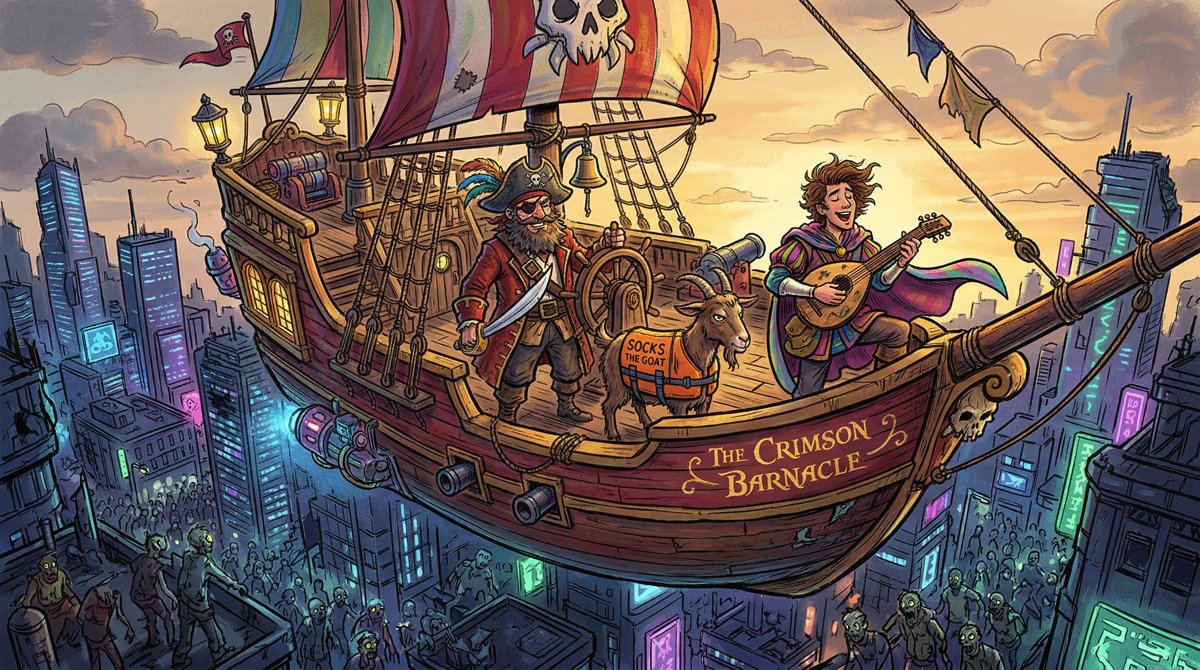
Orpheus, first mate and ship cook, speaks softly but firmly from the galley hatch. “You know the risks, Captain. If the TokPods get on the Crimson Barnacle, we may be lost ourselves.” Socks answers without looking away from the display. “We beat them once. Knowledge was the key.” Pete nods once. “Very well. Prepare to enter Earth’s atmosphere in Cloaking Mode.” Somewhere below, Hypno Hippo lounges on a throne of extracted attention, enormous and smug, feeding on outrage, dopamine drips, and the quiet death of critical thought.
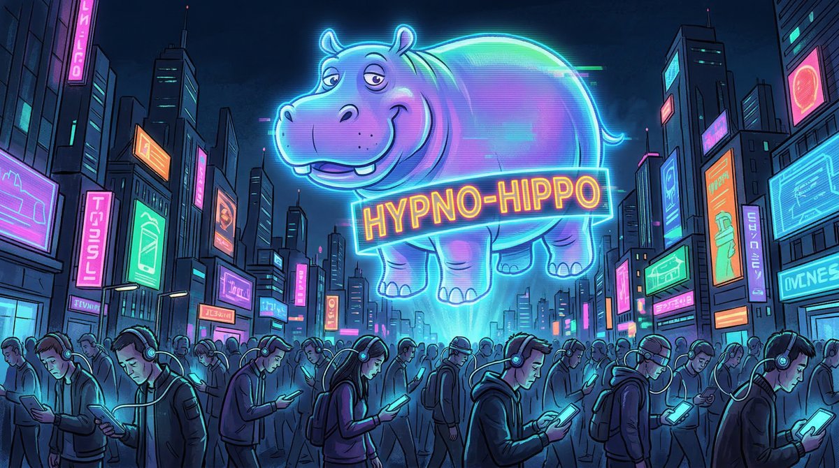
The crew’s plan is not a broadside of cannon. It is a hack of the feeds themselves: inject friction, teach trade-offs, and restore the one defense Hypno Hippo cannot hypnotize away—the ability to choose deliberately under scarcity. Through the lens of utility maximization, Brain-rot hours versus Economics Studying hours, the pirates will try to turn zombies back into humans. What follows is the economics they beam into the TokPod stream: how a fixed time budget, a slope you can calculate without fear, and the patient logic of marginal utility can break a planetary addiction.
1. Scarcity, Utility, and Why the Zombies Cannot Have It All
What “utility” actually means when your brain is on fire
Utility is the satisfaction, happiness, or goal-achievement a person gets from a choice. It is not a moral judgment and it is not “usefulness” in the engineering sense. A TokPod doom-scroll can deliver utility in the form of a dopamine hit; an hour of careful economics study can deliver utility in the form of clarity, exam points, and the long-run power to see through Hypno Hippo’s tricks. Cowen and Tabarrok treat utility as the economist’s placeholder for “whatever the decision maker is trying to get more of,” ranked consistently enough that we can talk about more and less [1]. The zombies of 2030 still have preferences. The tragedy is that the TokPod interface has scrambled their ability to notice the trade-offs those preferences imply.
Socks puts it to Stella Starlight, the dreamy third-class goat they once pulled from the North Atlantic, in the simplest possible frame. “Stella, you have one evening. Sixteen waking hours if we are generous. Every hour you feed the TokPod is an hour you do not spend learning how markets and budgets work. That missing hour is the opportunity cost.” Stella blinks. “So utility is… the good feeling from either one?” “Yes,” says Socks. “And because time is scarce, you cannot max both feelings at once. You have to choose a mix.”
Scarcity is the planet-wide precondition
Scarcity means human wants exceed the resources available to satisfy them. Time is the cleanest scarce resource in this episode: nobody mints extra hours. Becker’s classic framing treats households as producers who combine time and goods to create satisfaction; the same logic applies to a student choosing between Brain-rot (\(B\)) and Economics Studying (\(E\)) [2]. When the crew hacks the TokPod feed, the first sentence they burn onto every lock screen is: You cannot do everything. Choose on purpose.
Why Hypno Hippo hates this lecture
Hypno Hippo’s business model is freemium addiction: start free, deepen the feed, extract attention, then money, then the capacity to notice extraction. Critical thinking is his Achilles’ heel precisely because critical thinking is the comparison of marginal benefits and marginal costs under a hard budget. If the zombies re-learn that an hour has a price denominated in forgotten skills, the trance cracks. Petunia Pareto, floating near the nav console and muttering about derivatives, adds: “If we can get them to an interior optimum where the last bit of Brain-rot joy per minute equals the last bit of Study joy per minute, Hypno loses the extensive margin. They stop giving him everything.”
The rest of this lecture is the toolkit the crew uploads: a budget constraint in time, a slope you can compute by hand, diminishing marginal utility, and the equimarginal principle that pins down the best affordable bundle.
2. The Time Budget Constraint: Brain-Rot versus Economics Studying
Writing the constraint the way Orpheus writes a recipe
Orpheus refuses to skip steps. “If you cannot measure the flour,” he says, “you cannot bake the bread. Same with hours.” Let \(T\) be total available time in a study window (say, a 10-hour block the crew forces open by throttling TokPod push alerts). Let \(B\) be hours of Brain-rot and \(E\) be hours of Economics Studying. The linear time budget constraint is simply that the two uses add up to the total:
Every feasible plan sits on or inside that line. Points beyond it are fantasy—Hypno Hippo’s favorite product category.
Sometimes we write the same idea with explicit “prices” in time. If one hour of Brain-rot costs one hour of clock time and one hour of Studying costs one hour of clock time, the prices are \(P_B = 1\) and \(P_E = 1\), and total “money” is just total hours \(M = T\). The general goods form students will see in every textbook is:
For our pirate problem, \(X = B\), \(Y = E\), \(P_X = P_Y = 1\), \(M = T\). Later, when opportunity costs stop being one-for-one (for example, if “effective” study requires more focus per clock hour), the prices diverge and the line rotates. That is deliberate foreshadowing for demand.
Building the table by subtracting from the total (no steps skipped)
Simplified example: suppose the crew carves out a \(T = 10\) hour evening for a recovered zombie named Sam. Sam can put any whole number of hours into Brain-rot; the rest must go to Economics Studying (or idle rest, which we fold into “not studying with intent,” but here we keep two goods clean).
| Brain-rot hours \(B\) | Studying hours \(E = 10 - B\) | Bundle label |
|---|---|---|
| 0 | 10 | All study |
| 2 | 8 | Mostly study |
| 4 | 6 | Balanced-lean-study |
| 5 | 5 | Fifty-fifty |
| 6 | 4 | Balanced-lean-rot |
| 8 | 2 | Mostly rot |
| 10 | 0 | All TokPod |
Set notation helps when we talk about the whole menu of options. The feasible set is all pairs \((B, E)\) such that \(B \geq 0\), \(E \geq 0\), and \(B + E \leq 10\). The budget line itself is the boundary \(B + E = 10\). Interior points (for example, 3 hours rot, 3 hours study, 4 hours pure sleep) are feasible but will not be chosen if both activities yield positive marginal utility and sleep has already been optimized elsewhere—another Orpheus reminder not to hide assumptions.
Finding the intercepts without panic
The B-intercept is where Studying is zero: set \(E = 0\) in Eq. 1, so \(B = T = 10\). Graphically that is the point \((10, 0)\) if \(B\) is on the horizontal axis and \(E\) on the vertical. The E-intercept is where Brain-rot is zero: \(B = 0\), so \(E = 10\), the point \((0, 10)\). Stella asks the clueless-but-crucial question: “Why do we care about corners?” Socks: “Because intercepts tell you the maximum of one good if you abandon the other. They are the ‘all-in’ threats Hypno Hippo wants you to make without noticing.”
Sam’s 10-hour time budget: Brain-rot vs Economics Studying
Straight budget line from (0,10) to (10,0) showing all combinations of Brain-rot and Studying hours that sum to 10. Hover labels name the corner and midpoint bundles.
3. Slope, Opportunity Cost, and Reading the Line Like a Navigator
Slope is rise over run—said slowly
The slope of a straight line is the change in the vertical variable divided by the change in the horizontal variable. On our budget line, when Brain-rot rises by \(\Delta B\), Studying must fall by \(\Delta E\) to keep \(T\) fixed. From Eq. 1, \(\Delta E = - \Delta B\) when \(T\) is fixed and prices are one. So:
With \(P_B = P_E = 1\), the slope is \(-1\). That number is not decoration. It is the opportunity cost of one more hour of Brain-rot, measured in hours of Studying sacrificed. Socks walks Stella through a numerical move: start at \((B,E) = (4,6)\). Add 2 hours of TokPod. New point: \((6,4)\). Rise is \(4 - 6 = -2\). Run is \(6 - 4 = +2\). Slope \(= (-2)/(+2) = -1\).
Slope between (4,6) and (6,4) on the T=10 budget
\(\frac{E_2 - E_1}{B_2 - B_1}\)
| Input | Value | Unit |
|---|---|---|
| E1 (study hours at start) | 6 | hours |
| E2 (study hours at end) | 4 | hours |
| B1 (rot hours at start) | 4 | hours |
| B2 (rot hours at end) | 6 | hours |
Result: -1 study hours per rot hour
Relative prices and the price ratio
In the two-goods money model, the absolute value of the budget slope equals the price ratio:
On the time budget with equal time prices, the ratio is 1—one study hour per rot hour. If the crew later makes Brain-rot “more expensive” in effective attention (say, by adding friction so that each clock hour of TokPod burns more recovery time), \(P_B\) rises relative to \(P_E\) and the line rotates. Section 6 returns to that rotation; it is how we will eventually derive demand.
Check yourself: If T = 8 hours and Sam moves from (1,7) to (5,3), what is the slope, and what opportunity cost does it encode?
Rise = \(3 - 7 = -4\). Run = \(5 - 1 = +4\). Slope = \(-1\). Each added Brain-rot hour still costs one Studying hour. The opportunity cost per hour of rot is 1 hour of study; the slope of the budget line is \(-1\).
Parallel shifts when the time endowment changes
If the crew wins a bigger window—say exam week protections push \(T\) from 10 to 12—the intercepts both move out to 12 and the new line is parallel to the old one (same slope \(-1\)). More total time is like a higher income in the goods model: you can afford more of both activities. A parallel inward shift (TokPod emergency alerts eating the evening) shrinks both intercepts.
Parallel shifts of the time budget when T changes
Three parallel budget lines with slope -1: T=7, T=10, and T=12. Parallel shifts show pure endowment changes without changing relative opportunity cost.
Dino Ambrosi’s short film 4000 hours makes the same scarcity visceral at life scale: the finite stack of hours between a young adult and a long goal [3]. The pirates pipe a cut of it into the TokPod stream between utility diagrams—not as guilt, but as a clock. Tavčar’s 4000 pushes a related meditation on attention and finite life [4]. The micro model here is the daily version of that stack: \(T = B + E\) on one evening is practice for \(T\) across a life.
4. Marginal Utility, Diminishing Returns, and Why the Tenth Video Hits Different
Total utility versus marginal utility
Total utility is the overall satisfaction from a bundle. Marginal utility (\(MU\)) is the extra satisfaction from one more unit of a good, holding the other good fixed. If Sam’s total utility from Studying hours runs 0, 20, 36, 48, 56, 60 as \(E\) goes 0 through 5 (simplified teaching numbers), then the marginal utilities are the differences: 20, 16, 12, 8, 4. The crew’s teaching feed flashes:
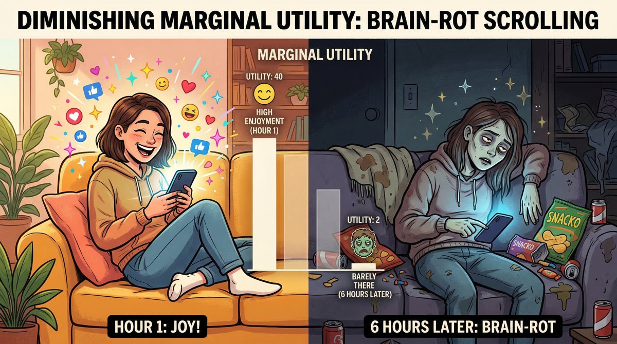
Diminishing marginal utility (the shape Hypno Hippo exploits and fears)
Diminishing marginal utility says that as you consume more of one good, holding the other fixed, the extra satisfaction from additional units eventually falls. The first hour of Brain-rot after a brutal day can feel huge. The seventh hour in a row often feels numb—yet the autoplay continues, because the interface hides the comparison to what Studying’s next hour would have been worth. Economics Studying diminishes too: the first focused hour can unlock a concept; the fifth fatigued hour may add little. Diminishing MU is not a moral failing. It is a regularity that makes interior bundles attractive instead of corners.
Indifference curves in the Brain-rot / Study plane
An indifference curve connects bundles that yield the same utility. Higher curves (up and right, when both goods are goods) mean more utility. They do not cross if preferences are transitive. The slope of an indifference curve is the negative of the marginal rate of substitution (MRS)—how much Studying Sam will give up for one more rot hour while staying equally happy:
(Here \(X = B\), \(Y = E\).) When \(MU_B\) is high relative to \(MU_E\), Sam will trade a lot of study for a little more rot and still feel whole; the curve is steep in absolute value depending on axis choice. As Sam moves toward rot-heavy bundles, diminishing \(MU_B\) and rising \(MU_E\) (because study became scarce) flatten the willingness to pay for still more rot.
Indifference curves for Brain-rot vs Studying (conceptual)
Three convex-to-the-origin indifference curves in Brain-rot–Studying space. Higher curves represent higher utility. Shape reflects diminishing MRS.
5. Utility Maximization: Where the Budget Touches the Highest Curve
The tangency picture
Sam wants the highest indifference curve that still touches the budget set. With smooth curves and an interior solution, that happens where the indifference curve is tangent to the budget line—same slope. Budget slope magnitude is the price ratio; indifference slope magnitude is the MRS. So utility maximization requires:
which is the same information as the equimarginal principle:
In words: the last hour’s worth of satisfaction per unit of scarce time should match across uses. If Brain-rot still yields more MU per hour than Studying, Sam should reallocate toward rot; if Studying yields more MU per hour, reallocate toward study. Stop when the two “bangs per buck” (here, bangs per hour) are equal—and the budget is exhausted.
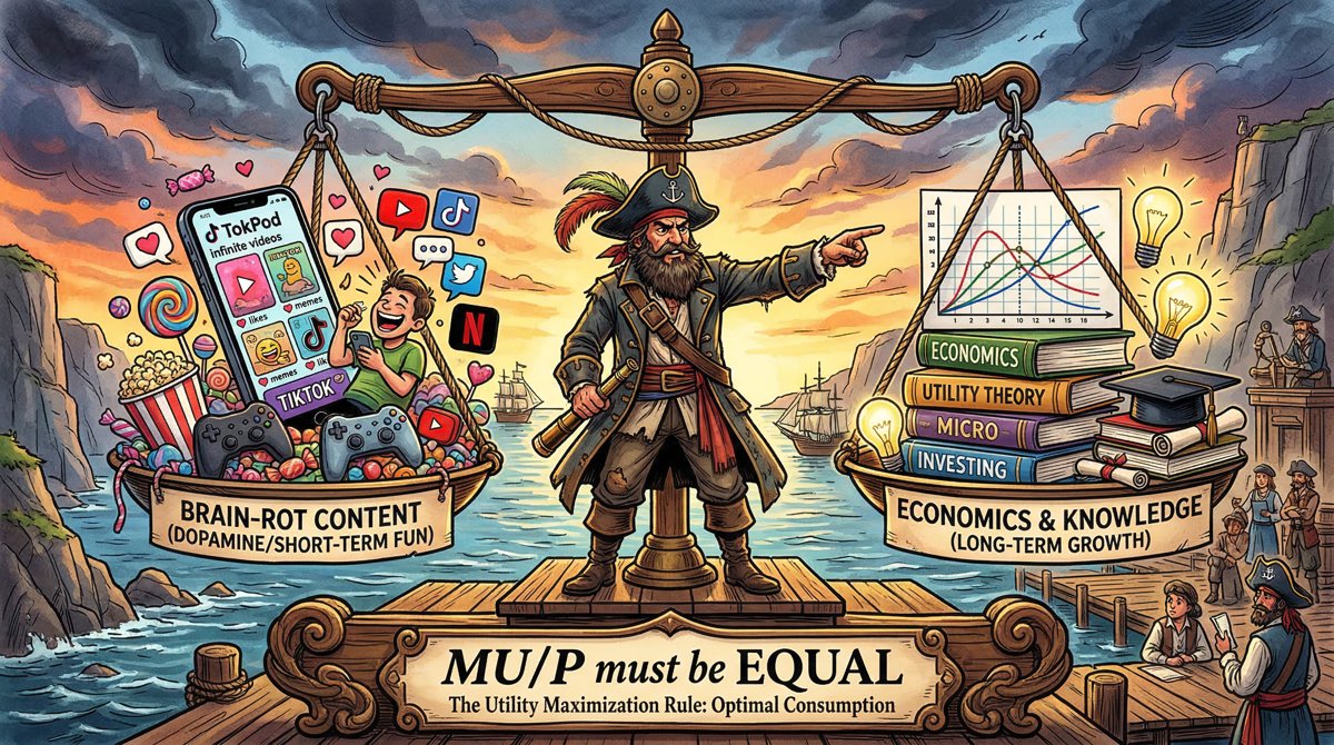
Why “utility is equal for all combinations” on a curve—but not across curves
On one indifference curve, every bundle is ranked the same; utility is constant by construction. Across curves, utility differs. Students sometimes hear “utility is equal” and think every bundle in life is the same. Petunia Pareto corrects gently: “Equal along the curve. The whole point of maximization is to climb to a higher curve without breaking the budget.”
Cobb–Douglas as a workhorse (parameters known, slope known)
Instructors often use a Cobb–Douglas utility function \(U = B^{\alpha} E^{1-\alpha}\) (or \(U = B^{a} E^{b}\)) because the math is friendly: the MRS simplifies to a clean function of the ratio \(E/B\), and the optimal expenditure shares become constants. Simplified example: let \(\alpha = 0.5\), so \(U = \sqrt{B} \sqrt{E} = \sqrt{BE}\). Then \(MU_B = \partial U/\partial B = \frac{1}{2}\sqrt{E/B}\) and \(MU_E = \frac{1}{2}\sqrt{B/E}\), so \(MRS = MU_B/MU_E = E/B\). Set MRS equal to the price ratio \(P_B/P_E = 1\):
With \(B + E = 10\), the unique interior optimum is \(B = 5\), \(E = 5\). You did not need a computer. You used the known preference parameter (equal exponents → equal time shares when prices are equal) and the known budget slope.
Cobb–Douglas time shares with equal exponents on a 10-hour budget
\(B^{*} = \alpha T,\; E^{*} = (1-\alpha) T\)
| Input | Value | Unit |
|---|---|---|
| alpha (exponent on Brain-rot) | 0.5 | share |
| T (total hours) | 10 | hours |
Result: 5 hours of B (and 5 of E)
Utility maximization: tangency at equal time shares
Budget line from (0,10) to (10,0) with a lower indifference curve that cuts the budget and a higher indifference curve tangent at (5,5), the utility-maximizing bundle under equal prices and equal Cobb–Douglas weights.
Check yourself: If MU_B = 12, MU_E = 6, and time prices are equal (P_B = P_E = 1), is Sam maximizing? Which way should hours move?
Compute \(MU_B/P_B = 12\) and \(MU_E/P_E = 6\). Not equal. The bang per hour is higher for Brain-rot, so Sam should move toward more \(B\) and less \(E\) until diminishing MU brings the ratios together (and the budget still binds). If this seems to endorse addiction, remember: the MU numbers are Sam’s current feelings—often inflated by interface design. Part of the crew’s hack is helping Sam measure MU more honestly after friction is added.
6. Shifts versus Rotations: Changing Relative Opportunity Costs
Parallel shift recap (endowment only)
When \(T\) changes and both time prices stay 1, intercepts move equally and slope stays \(-1\). That is a pure income-style effect in time space. Recovered zombies with longer protected study blocks can reach higher indifference curves even with the same preferences.
Rotation when relative prices change
Now suppose the crew’s friction tech makes each clock hour of Brain-rot cost two hours of effective recovery and attention debt, while Studying still costs one. In an effective-time budget, \(P_B = 2\), \(P_E = 1\), and if the “real” resource is 10 effective hours, the constraint reads \(2B + E = 10\). Intercepts: if \(B = 0\), \(E = 10\); if \(E = 0\), \(B = 5\). Slope \(\Delta E / \Delta B = -P_B/P_E = -2\). The line is steeper. Opportunity cost of rot just doubled.
Rotating the time budget when relative opportunity costs change
Three budget lines sharing conceptual endowment but different relative prices: slope -1 baseline, slope -2 when Brain-rot becomes more costly, slope -0.5 when Studying becomes more costly. Rotations change opportunity cost; they are not parallel shifts.
Simplified example with Cobb–Douglas \(\alpha = 0.5\) again: equal exponents still want equal expenditure shares. Expenditures are \(P_B B\) and \(P_E E\). With \(P_B = 2\), \(P_E = 1\), \(M = 10\), equal shares mean \(2B = 5\) and \(E = 5\), so \(B = 2.5\), \(E = 5\). Check the budget: \(2(2.5) + 5 = 10\). Check equimarginal logic: quantities adjust until MU per dollar matches. Relative to the old \((5,5)\) point, rot falls hard when its price rises. **That quantity response is the seed of a demand curve.**
New optimum after Brain-rot time-price doubles (Cobb–Douglas α=0.5)
\(B^{*} = \frac{\alpha M}{P_B}\)
| Input | Value | Unit |
|---|---|---|
| alpha | 0.5 | share |
| M (effective hours) | 10 | hours |
| P_B | 2 | effective hours per rot hour |
Result: 2.5 hours of Brain-rot
Policy toolkit in one image
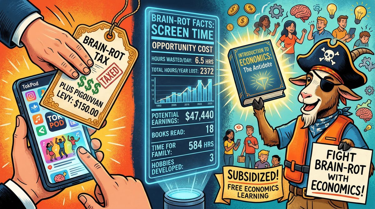
The crew’s broader intervention map—friction on feeds, protected study blocks, default opt-outs, literacy nudges—sits in their field manual as a single schematic. Each tool is either a shift (more total usable time) or a rotation (higher relative cost of rot) or a preference change (education that alters MU schedules themselves).
7. From Tonight’s Optimum to Tomorrow’s Demand Curve
Holding preferences fixed, vary the price of Brain-rot
Deriving demand from utility means: repeat the maximization for many values of \(P_B\), record the optimal \(B^{*}(P_B)\), and plot quantity of rot on the horizontal axis against price on the vertical. With Cobb–Douglas shares, \(B^{*} = \alpha M / P_B\)—a rectangular hyperbola shaped demand when \(\alpha\) and \(M\) are fixed. Even without a formula, the geometric story is stable: as the budget line steepens against rot, the tangency typically slides toward less \(B\).
Socks navigates Stella through three prices mentally: cheap rot → lots of rot at the tangency; expensive rot → little rot; absurdly expensive rot → near-zero rot, almost all study. “That downward map,” Socks says, “is demand. Markets will need it when we hit the Paper Toilet Shortage arc and the mercantilist spice markets. Tonight is the personal trailer for that movie.”
Time-use literacy as resistance
Becker’s allocation-of-time framework was never only about wages and housework; it is a reminder that every human day is a constrained optimization—whether or not the human writes a Lagrangian [2]. The TokPod zombie crisis is what happens when an interface optimizes against you, harvesting the residual you stop optimizing for yourself. Utility maximization, taught slowly enough that slope is no longer scary, is not a celebration of cold calculation. It is how the Crimson Barnacle gives people their agency back one evening budget at a time.
What the crew cannot do for you
They cannot feel your MU schedule. They cannot pick your \(\alpha\). They can only force the feed to show the constraint, the slope, and the equalizing rule. Trillionare Bob and Vilfredo Vitriol, elsewhere in the timeline, will try to scramble initial allocations and call the scramble destiny. Petunia Pareto will answer that efficiency talk without honesty about constraints is another trance. For this episode, the win condition is smaller and sharper: a student who can build the table, plot the intercepts, compute the slope, and say out loud whether \(MU_B/P_B\) still exceeds \(MU_E/P_E\).
Key Takeaways
- Scarcity forces trade-offs; the daily form in this episode is \(T = B + E\) between Brain-rot and Economics Studying.
- A budget constraint shows all affordable bundles; intercepts are “all-in” extremes, and slope encodes opportunity cost (with a minus sign on the graph).
- Utility ranks satisfaction; marginal utility is the extra from one more unit; diminishing marginal utility makes balanced bundles attractive.
- Utility maximization (interior) occurs where \(MU_B/P_B = MU_E/P_E\)—the equimarginal principle—equivalently where MRS equals the price ratio (tangency).
- Parallel shifts come from endowment changes; rotations come from relative-price changes and set up deriving demand from utility.
- Cobb–Douglas with known exponents plus a known budget slope yields an exact Umax bundle without hand-waving—building numeracy on purpose.
- Hypno Hippo’s trance thrives on hidden constraints; graphing the constraint is an act of resistance, not just homework.
Practice Problems
- Scenario: Mira has a 6-hour evening after work. Brain-rot and Studying are the only two uses, each costing one hour per hour.
Ask: Write the budget equation, find both intercepts, and compute the slope between \((1,5)\) and \((4,2)\).
Show answer
Budget: \(B + E = 6\). B-intercept \((6,0)\); E-intercept \((0,6)\). Slope \((2-5)/(4-1) = (-3)/3 = -1\). Opportunity cost of one rot hour is one study hour.
- Scenario: Same 6-hour budget. Simplified MU schedule at Mira’s current bundle: \(MU_B = 10\), \(MU_E = 30\), prices both 1.
Ask: Is she maximizing? Which way should she reallocate, and which principle are you using?
Show answer
\(MU_B/P_B = 10\), \(MU_E/P_E = 30\). Not equal. Studying yields more utility per hour, so shift time from Brain-rot toward Studying until the ratios equalize. Equimarginal principle Eq. 7.
- Scenario: Cobb–Douglas preferences with \(\alpha = 0.25\) on Brain-rot, \(1-\alpha = 0.75\) on Studying, \(T = 8\), prices equal to 1.
Ask: Find the utility-maximizing \((B^{*}, E^{*})\).
Show answer
Equal prices ⇒ expenditure shares equal weight shares: \(B^{*} = 0.25 \times 8 = 2\), \(E^{*} = 6\). Check: \(2 + 6 = 8\).
``calc { "title": "Cobb–Douglas optimum for Problem 3", "formula": "B^{*} = \\alpha T", "cite": "@cowen2024", "inputs": [ { "label": "alpha", "value": 0.25, "unit": "share" }, { "label": "T", "value": 8, "unit": "hours" } ], "result": { "value": 2, "unit": "hours of Brain-rot (E=6)" } } ``
- Scenario: The crew doubles the effective price of Brain-rot to \(P_B = 2\), \(P_E = 1\), effective endowment \(M = 8\), same \(\alpha = 0.25\).
Ask: Find the new \(B^{*}\). Did the budget shift parallel or rotate? What happens to rot hours versus problem 3?
Show answer
\(B^{*} = \alpha M / P_B = 0.25 \times 8 / 2 = 1\). The budget rotated (slope becomes \(-2\)), not parallel-shifted. Brain-rot hours fall from 2 to 1. That price–quantity pair is one point on Mira’s demand for rot.
Discussion Questions
- When the Crimson Barnacle adds friction to TokPod feeds, is that best modeled as a parallel shift of Sam’s time budget, a rotation, a change in the MU schedule, or a mix—and how would you defend your modeling choice with the episode’s images of Hypno Hippo’s business model?
- Stella Starlight asks clueless-sounding questions that force Socks to explain slope from scratch. Which step in building the Brain-rot / Studying graph (table, intercepts, rise/run, set notation) is hardest for you, and how does skipping that step help an attention-harvesting interface win?
- Petunia Pareto cares about welfare and efficiency; Vilfredo Vitriol wants to scramble initial allocations to his benefit. How does a population that never learns the equimarginal rule become easier for Vitriol-style villains to exploit, even if TokPods disappear?
- Ambrosi’s 4000 hours zooms out from one evening to a life. How does treating a single night’s \(T = B + E\) carefully train the same muscle you need for long-horizon time use—and where does diminishing marginal utility caution you against both pure grind and pure rot?
Glossary
- utility
- A measure of satisfaction or preference ranking a decision maker gets from a bundle of goods or activities.
- scarcity
- The condition that wants exceed the resources available to satisfy them, forcing trade-offs.
- trade-offs
- Giving up some of one thing to gain more of another when resources are limited.
- opportunity cost
- The value of the next-best alternative forgone when a choice is made.
- budget constraint
- The set of bundles that exhaust (or do not exceed) available income or time given prices.
- marginal utility
- The additional satisfaction from consuming one more unit of a good, holding other goods fixed.
- diminishing marginal utility
- The tendency for successive units of a good to add less extra satisfaction as quantity rises.
- equimarginal principle
- The rule that utility is maximized when marginal utility per unit of cost is equalized across goods.
- price ratio
- The relative price of two goods, Px/Py, which sets the magnitude of the budget line’s slope.
- feasible set
- All bundles that satisfy the budget constraint and nonnegativity; the affordable menu.
References
- Tyler Cowen and Alex Tabarrok. (2024). Modern Principles: Microeconomics. Worth Publishers/Macmillan
- Gary S. Becker. (1965). A Theory of the Allocation of Time. The Economic Journal. https://doi.org/10.2307/2228949
- Dino Ambrosi. (2023). 4000 hours. https://youtu.be/4TMPXK9tw5U?si=hJlvEjoO0BCGvGlE
- Ivan Tavčar. (2023). 4000. ZRC SAZU, Založba ZRC. https://doi.org/10.3986/9789610507000